T-distributed stochastic neighbor embedding

T-sne is a Latent Space visualization / dimensionality reduction technique particularly well-suited for high-dimensional data. It focuses on preserving local structures in the data, making it effective for visualizing clusters and patterns.

In Layman’s terms, it does this by computing the nearest neighbors of each point in the high dimensional space, and attempting to fine tune a model in the low dimensional space that matches these distances, such that points that were close in high-dim space remain close in low-dim space. The main difference between this (SNE) and t-SNE is that t-SNE uses a heavy-tailed distribution (Student t-distribution) in the low-dimensional space to better handle the “crowding problem”, where points tend to cluster too closely together. In addition, it makes the algorithm more efficient to compute(however, still extremely computationally expensive for large datasets).

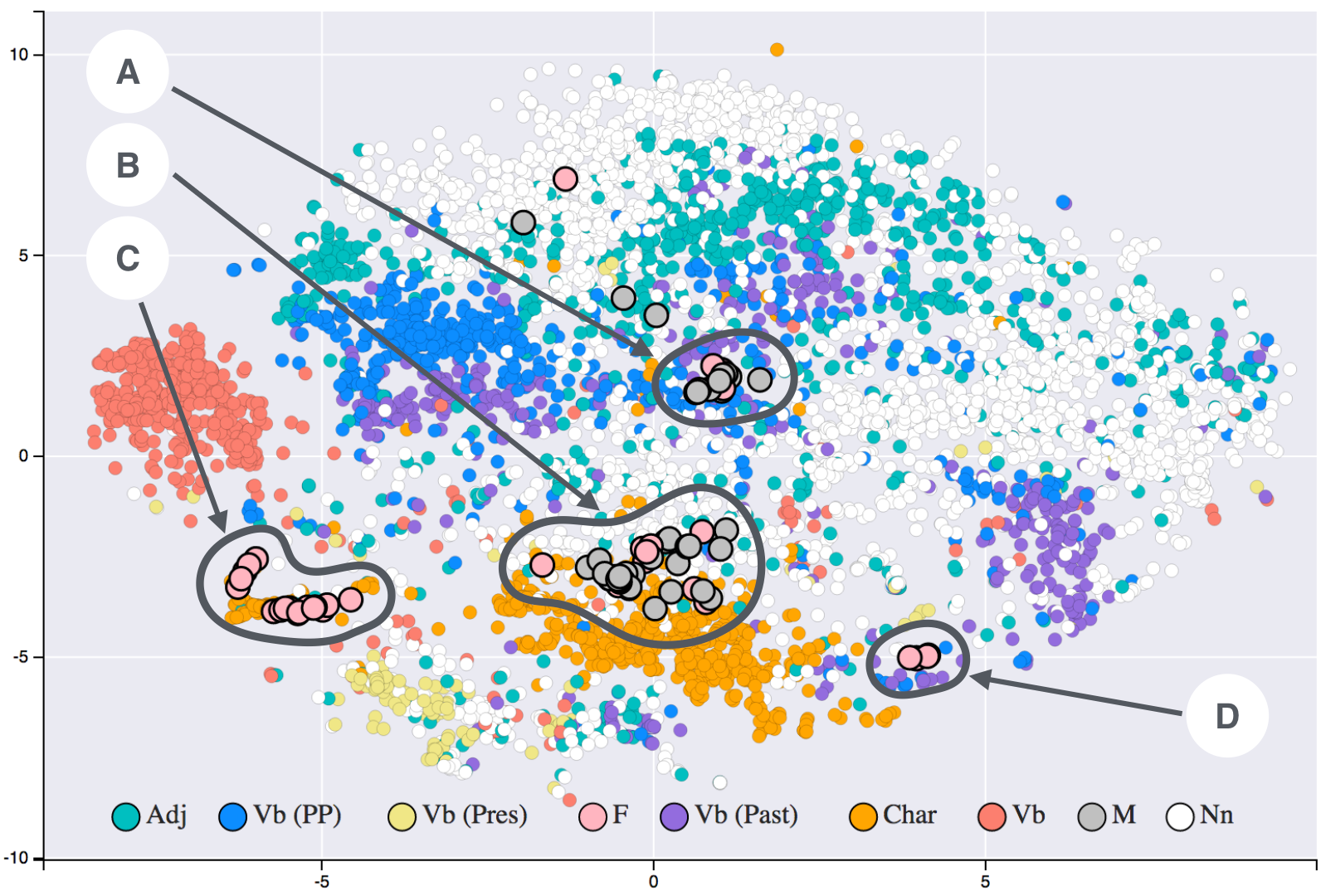
T-SNE applied to a 19th century word embeddings dataset, showing how words with similar meanings cluster together.

---

Formulation

High-Dim Similarities

T-SNE first computes pairwise similarities in the original high-dimensional space using a Gaussian distribution. The conditional probability that point $x_i$ would pick $x_j$ as its neighbor is:

$$p_{j|i}=\frac{\exp (-||x_i-x_j|{|}^2/2{\sigma }_i^2)}{{\sum }_{k\ne i}\exp (-||x_i-x_k|{|}^2/2{\sigma }_i^2)}$$

where ${\sigma }_i$ is the variance of the Gaussian centered on $x_i$. This variance is determined by the perplexity parameter.

To make the similarity metric symmetric, we use:

$$p_{ij}=\frac{p_{j|i}+p_{i|j}}{2n}$$

Low-Dim Similarities

In the low-dimensional map, t-SNE uses a Student t-distribution with one degree of freedom (also known as the Cauchy distribution). This heavy-tailed distribution is key to avoiding the “crowding problem”:

$$q_{ij}=\frac{(1+||y_i-y_j|{|}^2{)}^{-1}}{{\sum }_{k\ne l}(1+||y_k-y_l|{|}^2{)}^{-1}}$$

where $y_i$ and $y_j$ are the low-dimensional representations of $x_i$ and $x_j$.

Optimization Objective

T-SNE minimizes the Kullback-Leibler divergence between these two distributions:

$$C=\text{KL}(P||Q)=\sum _i\sum _j{p}_{ij}\log \frac{p_{ij}}{q_{ij}}$$

The gradient of this cost function with respect to the low-dimensional points is:

$$\frac{\delta C}{\delta y_i}=4\sum _j(p_{ij}-q_{ij})(y_i-y_j)(1+||y_i-y_j|{|}^2{)}^{-1}$$

This gradient is optimized using gradient descent with momentum.

Perplexity and ${\sigma }_i$

The perplexity is related to the entropy of the conditional probability distribution:

$$\text{Perp}(P_i)=2^{H(P_i)}=2^{-{\sum }_j{p}_{j|i}{\log }_2{p}_{j|i}}$$

For each point $i$, a binary search finds the ${\sigma }_i$ that produces the desired perplexity. This means each point effectively has a different “bandwidth” depending on the local density of the data.

---

Intuition

How T-SNE works can be understood in two main steps:

1. Build a probability distribution over pairs of high-dimensional objects in such a way that similar objects have a high probability of being picked, while dissimilar points have an extremely small probability of being picked.
2. Then, define a similar probability distribution over the points in the low-dimensional map, and minimize the Kullback-Leibler divergence between the two distributions with respect to the locations of the points in the map.

A key parameter in T-SNE is perplexity, which can be thought of as a smooth measure of the effective number of neighbors. It influences how the algorithm balances attention between local and global aspects of the data. Lower perplexity values focus more on local structures, while higher values capture broader patterns.

The different perplexity values 5-100 and how they change the depiction of the data.

---

Limitations

While a great approximation for many dimension reduction tasks, T-SNE has a few key issues. Namely, it is completely non-deterministic, and is unable to generalize to new data like Principle Component Analysis. It is a “trained” model in the sense that it learns this data distribution specifically, and that also comes with the downside of computational complexity, $O(N^2)$. In addition, many features of the visualization have no inherent meaning, namely that the distances between different clusters hold no value, and the cluster sizes themselves are arbitrary

When To Use What

Use t-SNE when: You want to visualize high-dimensional data with focus on local structure and clustering patterns.

Use PCA when: You need deterministic results, global structure preservation, or the ability to transform new data.

Use UMAP when: You want fast computation with both local and global structure preserved and the ability to transform new data.