Principle Component Analysis is a Latent Space visualization technique for linear pattern extraction and dimensionality reduction. It transforms high-dimensional data into a lower-dimensional space while preserving as much variance as possible.
For a two dimensional example mapping onto a line, you can think of PCA as finding the best line to fold the data onto, such that the distance from the points to the line is minimized. That “line” is the largest principle component of the distribution:
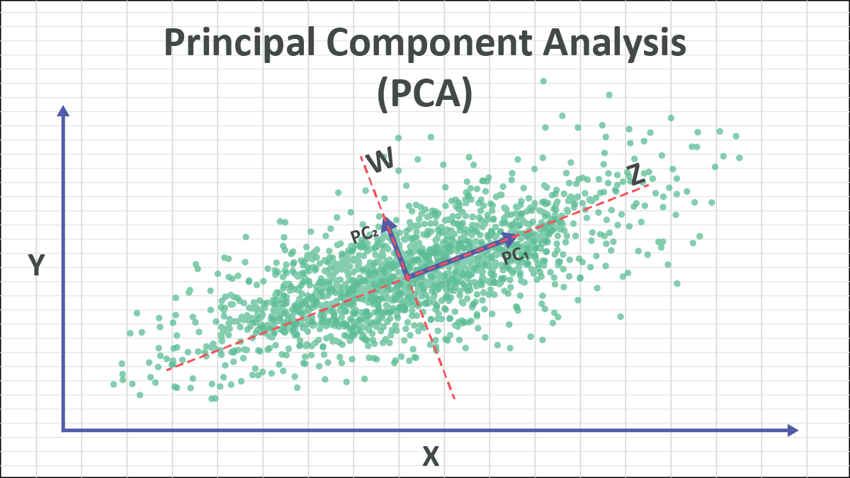
In the context of linear algebra, the Principle Component can be thought of as the eigenvector corresponding to the largest eigenvalue of the data’s covariance matrix. This eigenvector points in the direction of maximum variance in the data.
Computation
The first step in computing Principle Component Analysis is to find the covariance matrix.
This can be calculated by first centering your data, this means calculating the mean of every variable and then substracting that mean from each datapoint
And then calculating the Covariance matrix:
After obtaining the covariance matrix, the next step is to compute its eigenvalues and eigenvectors. The eigenvectors represent the directions of maximum variance (the principal components), while the eigenvalues indicate the magnitude of variance along those directions.
where:
- is an eigenvector
- is the corresponding eigenvalue
- is the covariance matrix of the dataset
These eigenvectors(our principle components) are then sorted in descending order based on their corresponding eigenvalues. The top eigenvectors (where is the desired number of dimensions) are selected to form a new feature space.
Finally, the original data is projected onto this new feature space by multiplying the centered data matrix by the matrix of selected eigenvectors:
For a dataset: