Linearization and the Jacobian

Linear maps describe local behavior of nonlinear systems. Near a fixed point, any smooth map looks linear. The Jacobian matrix(the derivative of a nonlinear map) is exactly this linear approximation. So understanding how linear maps behave (sinks, sources, saddles) directly tells us how a nonlinear system behaves near its fixed points.

This is the bridge between linear and nonlinear dynamics.

---

Linear Map Behavior

We are continuing from the previous lecture on Linear Maps. The key insight: eigenvalues determine everything. They tell us whether a region shrinks, expands, or does both (saddle):

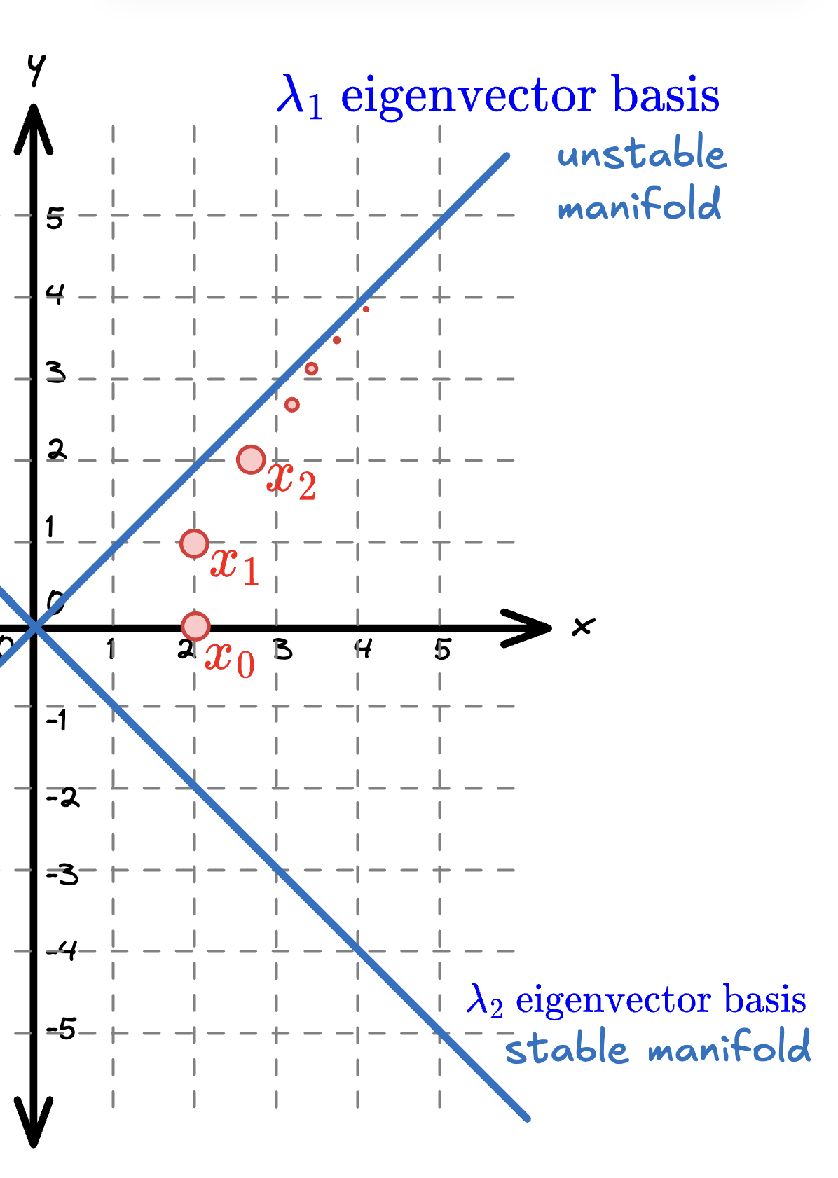
Starting from ${\vec{x}}_0=(2,0)$, successive iterations climb along the ${\lambda }_1$ eigenvector direction (unstable manifold). Since ${\lambda }_1=\frac{3}{2}>1$, points expand along this direction. The ${\lambda }_2$ eigenvector basis forms the stable manifold - points on this line contract toward the origin since ${\lambda }_2=\frac{1}{2}<1$.

The Hénon Map has two fixed points where we can compute these eigendirections:

$$(0,0)\text{and}(-0.6,-0.6)$$

---

Classification of Linear Maps

Linear maps on ${\mathbb{R}}^2$ come in three flavors (up to a change of coordinates to eigenvector basis). The eigenvalues determine which type, and we’ll see that each type produces fundamentally different dynamics:

Type 1: Distinct Real Eigenvalues

$$A=\left[\begin{array}{cc}a& 0\\ 0& b\end{array}\right]$$

The matrix is diagonal in eigenvector coordinates. Different eigenvalues mean different expansion rates in different directions, this is how saddles are born.

Maps the unit disc to an ellipse with semi-major axes of length $|a|$ (x-axis) and $|b|$ (y-axis). Behavior depends on the magnitudes:

• If $|a|,|b|<1$: ellipse shrinks → sink
• If $|a|,|b|>1$: ellipse expands → source
• If $|a|>1>|b|$ or vice versa: ellipse stretches in one direction, contracts in another → saddle

Type 2: Repeated Real Eigenvalues

$$A=\left[\begin{array}{cc}a& 1\\ 0& a\end{array}\right]$$

Both eigenvalues are identical, so there’s no direction to expand while another contracts. No saddles here, as saddles require competing eigenvalues with different magnitudes.

Type 3: Complex Eigenvalues

$$A=\left[\begin{array}{cc}a& -b\\ b& a\end{array}\right]$$

Complex eigenvalues come in conjugate pairs $a\pm bi$ with equal magnitude $r=\sqrt{a^2+b^2}$. We can factor this as:

$$A=r\left[\begin{array}{cc}\cos \theta & -\sin \theta \\ \sin \theta & \cos \theta \end{array}\right]$$

where $\tan \theta =b/a$. This means $A$ rotates points by angle $\theta$ and scales them by factor $r$.

no saddle, rotation + uniform scaling together means no stretching in one direction while contracting in another.

---

Theorem

Let $A$ be a linear map on ${\mathbb{R}}^m$ represented by a matrix. Then:

1. The origin is a sink if all eigenvalues satisfy $|\lambda |<1$
2. The origin is a source if all eigenvalues satisfy $|\lambda |>1$
3. The origin is a saddle if $A$ is hyperbolic (no eigenvalues with $|\lambda |=1$) with mixed magnitudes: at least one $|\lambda |>1$ and at least one $|\lambda |<1$

---

Linearizing Nonlinear Maps: The Jacobian

But most dynamical systems are nonlinear. The Hénon Map is nonlinear: $f(x,y)=(1-x^2+by,x)$. How do we use our eigenvalue theory here?

Near a fixed point $\vec{p}$, a nonlinear map behaves like a linear map. The matrix that captures this linear behavior is the Jacobian matrix, matrix of partial derivatives.

---

Computing the Jacobian

Let $\vec{f}=(f_1,f_2,\dots ,f_m)$ be a map on ${\mathbb{R}}^m$ and let $\vec{p}\in {\mathbb{R}}^m$. The Jacobian matrix of $\vec{f}$ at $\vec{p}$, denoted $\mathcal{D}\vec{f}(\vec{p})$ is given by the matrix of Partial Derivatives of $\vec{f}$ evaluated at $\vec{p}$.

$$\mathcal{D}\vec{f}(\vec{p})=\left[\begin{array}{ccccc}\frac{\partial f_1}{\partial x_1}(\vec{p})& \frac{\partial f_1}{\partial x_2}(\vec{p})& \dots & \frac{\partial f_1}{\partial x_n}(\vec{p})& \\ \frac{\partial f_2}{\partial x_1}(\vec{p})& \frac{\partial f_2}{\partial x_2}(\vec{p})& \dots & \frac{\partial f_2}{\partial x_n}(\vec{p})& \\ ⋮& ⋮& ⋮& ⋮& \end{array}\right]$$

Example

Henon Map $f(x,y)=(a-x^2+by,x)$

$$\mathcal{D}\vec{f}(x,y)=\left[\begin{array}{cc}-2x& b\\ 1& 0\end{array}\right]$$

Why Does This Work?

We will look at uses of the Taylor Series next class, heres a snippet

$$(in{\mathbb{R}}^1):f(x+h)=f(x)+f^{\prime }(x)h+f^{\prime \prime }(x)\frac{h^2}{2!}+\dots$$ $$\vec{f}(\vec{p}+\vec{h})=f(\vec{p})+\mathcal{D}\vec{f}(\vec{p})$$