15.3 - Double Integrals in Polar Coordinates

Many integration regions can be described conveniently in polar coordinates. Recall the meaning of the polar coordinate $(r,\theta )$

MatPlotLib Example

import matplotlib.pyplot as plt
import numpy as np
 
# Values for demonstration (r = distance, theta = angle in radians)
r = 5  # radial distance
theta = np.pi / 4  # 45 degrees
 
# Convert from polar to cartesian coordinates
x = r * np.cos(theta)
y = r * np.sin(theta)
 
# Create figure and axis
fig, ax = plt.subplots()
 
# Plot the line representing (r, theta)
ax.plot([0, x], [0, y], 'brown', label=r'$\theta$ line')
ax.plot([x, x], [0, y], 'k--')  # dashed line representing height (y)
ax.plot([0, x], [y, y], 'k--')  # optional horizontal line for x
 
# Plot the point at (r, theta)
ax.plot(x, y, 'bo')  # blue point at the end
 
# Annotations for polar coordinates (r, θ)
ax.annotate(r'$r = \mathrm{Distance\ from\ Pole}$', xy=(x / 2, y / 2), xytext=(-5, 1.5),
            textcoords='offset points', fontsize=12, color='brown')
ax.annotate(r'$\theta = \mathrm{Polar\ Angle}$', xy=(x / 2, y / 2), xytext=(15, -10),
            textcoords='offset points', fontsize=12, color='purple')
 
# Annotations for Cartesian coordinates (x, y)
ax.annotate(r'$(r, \theta)$', xy=(x, y), xytext=(5, 5),
            textcoords='offset points', fontsize=12, color='blue')
ax.annotate(r'$x$', xy=(x, 0), xytext=(5, -10), textcoords='offset points', fontsize=12)
ax.annotate(r'$y$', xy=(0, y), xytext=(-15, 0), textcoords='offset points', fontsize=12)
 
# Set axis limits and labels
ax.set_xlim(0, r + 1)
ax.set_ylim(0, r + 1)
ax.set_aspect('equal', 'box')
 
# Axes labels
ax.set_xlabel('x')
ax.set_ylabel('y')
 
# Add the origin label
ax.text(-0.5, -0.5, 'Pole / Origin', fontsize=10)
 
# Show the grid and plot
ax.grid(True)
plt.title('Polar Coordinates vs Cartesian Coordinates')
plt.show()

Relationship to Cartesian:

$$x=r\cos \theta$$ $$y=r\sin \theta$$ $$x^2+y^2=r^2$$

---

Polar Coordinate Examples

Here are some sketched examples of polar coordinates:

Sketch

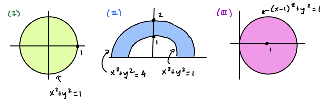
1. The disk $x^2+y^2\ge 1;\{(r,\theta ):0\le r\le 1,0\le \theta \le 2\pi \}$
2. The semi-annulus $1\le x^2+y^2\le 4;\{(r,\theta ):1\le r\le 2,0\le \theta \le \pi \}$
3. The disk $(x-1{)}^2+y^2\le 1;\left\{(r,\theta ):0\le r]leq2\cos \theta ,\frac{-\pi }{2}\le \theta \le \frac{\pi }{2}\right\}$

The circle in the third example is given by:

Expanding and Simplifying:

$$(x-1{)}^2+y^2=1\to x^2-2x+1+y^2=1$$ $$\to x^2+y^2=2x$$

Using conversion $x^2+y^2=r^2$ and $x=r\cos \theta$

$$\to r^2=2r\cos \theta$$ $$\to r=2\cos \theta$$

---

Double Integrals in Polar Coordinates

Suppose we wish to find the volume of the solid beneath the surface $z=f(x,y)$ and above the region $\mathcal{D}$, where $\mathcal{D}$ is described in polar coordinates. We seek:

$$\int {\int }_{\mathcal{D}}f(x,y)dA=\int {\int }_{\mathcal{D}}f(r\cos \theta ,r\sin \theta )dA$$

where we have made the substitution $x=r\cos \theta$, $y=r\sin \theta$, and $dA$ represents the area element in polar coordinates. To determine the area element, we must understand what it means to integrate over a polar region. The general polar region given by $\mathcal{D}$, where

$$\mathcal{D}=\{(r,\theta ):a\le r\le b,\alpha \le \theta \le \beta \}$$

represents the following sector:

Sketch

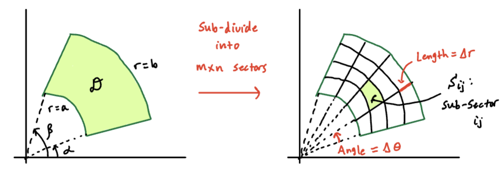
If we divide $[a,b]$ into $m$ sub-intervals of width $\Delta r=\frac{b-a}{m}$, and $[\alpha ,\beta ]$ into n sub-intervals of width $\Delta \theta =(\beta -\alpha )|n$, we obtain $m\times n$ sub-sectors (see the right-side of the above figure).

Let’s determine the area of a sub-sector:

Sketch

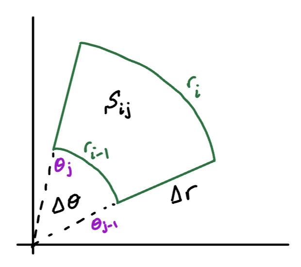
For very small $\Delta r$ and $\Delta \theta$, the sub sector is nearly a rectangle with height $\Delta r$ and width equal to the arc length of one side of the sector. If we choose the “long” side, the arc length is $r_i\Delta \theta$

Therefore:

$$Areaof{S}_{ij}=\Delta A=\Delta r\cdot r_i\Delta \theta =r{i}_i\Delta r\Delta \theta$$

When we take the ${\lim }_{m,n\to \infty }$, the polar area element is:

Polar Area Element

$$dA=rdrd\theta$$

Using this expression, we obtain the following:

Important

If $f$ is continuous on a “polar rectangle” $\mathcal{D}$ given by $a\le r\le b$, $\alpha \le \theta \le \beta$, then:

$$\int {\int }_{\mathcal{D}}f(x,y)dA={\int }_{\alpha }^{\beta }{\int }_a^{b}f(r\cos \theta ,r\sin \theta )rdrd\theta$$

Observe the extra factor of r that must be included!

---

Examples

Example

Evaluate:

$$\int {\int }_{\mathcal{D}}(3x+4y^2)dA$$

where $\mathcal{D}$ is the semi-annulus shown at the beggining, $1\le x^2+y^2\le 4$.

Solution

We integrate in polar coordinates with respect to $r$ and $\theta$, so we must determine bounds on $r$ and $\theta$. From the figure at the beggining, $\mathcal{D}$ can be described as:

$$\mathcal{D}=\{(r,\theta ):1\le r\le 2,0\le \theta \le \pi \}$$

We make the substitutions $x=r\cos \theta$, $y=\sin \theta$, $dA=rdrd\theta$, into the integrand to obtain:

$$\int {\int }_{\mathcal{D}}(3x+4y^2)dA={\int }_0^{\pi }{\int }_1^2(3r\cos \theta +4r^2{\sin }^2\theta )rdrd\theta$$ $$={\int }_0^{\pi }{\int }_1^{2}3r^2\cos \theta +4r^3{\sin }^2\theta drd\theta$$

Carry out the integration:

$$I_1:{\int }_1^{2}3r^2\cos \theta +4r^3{\sin }^2\theta dr={r^3\cos \theta +r^4{\sin }^2\theta |}_1^2$$ $$=8\cos \theta +16{\sin }^2\theta -\cos \theta -{\sin }^2\theta$$ $$=7\cos \theta +15{\sin }^2\theta$$ $$I_2:{\int }_0^{\pi }7\cos \theta +15{\sin }^2\theta d\theta ={\int }_0^{\pi }7\cos \theta +\frac{15}{2}(1-\cos 2\theta )d\theta$$

We use the half angle identity:

$$={7\sin \theta +\frac{15}{2}\theta -\frac{15}{4}\sin (2\theta )|}_0^{\pi }=\frac{15\pi }{2}$$

Remark

The half angle identities will be useful for these problems:

$${\cos }^2\theta =\frac{1+\cos (2\theta )}{2},{\sin }^2\theta =\frac{1-\cos (2\theta )}{2}$$

---

The Gaussian Integral

We will now prove the famous result:

$${\int }_{-\infty }^{\infty }{e}^{-x^2}dx=\sqrt{\pi }$$

This is the so-called Gaussian Integral

Proof

Observe that:

$${\int }_{-\infty }^{\infty }{\int }_{-\infty }^{\infty }{e}^{-(x^2+y^2)}dxdy={\int }_{-\infty }^{\infty }{e}^{-x^2}dx\cdot {\int }_{-\infty }^{\infty }{e}^{-y^2}dy$$

(*)

because we can write the first integrand as a product of two functions independent of each other. The improper integrals on the right-hand side have the same value, so (*) says:

$${\int }_{-\infty }^{\infty }{\int }_{-\infty }^{\infty }{e}^{-(x^2+y^2)}dxdy={\left({\int }_{-\infty }^{\infty }{e}^{-x^2}dx\right)}^2$$

(**)

We will compute. the double integral on the left-hand side with polar coordinates.

The integration region is $-\infty <x<\infty$, $-\infty <y<\infty$, i.e., the entire xy-plane. In polar coordinates, we can describe the xy-plane by $0\le \theta \le 2\pi$, $0\le r\le \infty$. The Double Integral becomes:

$${\int }_{-\infty }^{\infty }{\int }_{-\infty }^{\infty }{e}^{-(x^2+y^2)}dxdy={\int }_0^{2\pi }{\int }_0^{\infty }{e}^{-r^2}\cdot rdrd\theta$$

Solving with I1 and I2

$I_1:$ This is an improper integral of the first kind:

$${\int }_0^{\infty }r{e}^{-r^2}dr=\underset{t\to \infty }{\lim }{\int }_0^{t}r{e}^{-r^2}dr$$

Using U-sub: $u=r^2,du=2rdr,r\to \infty$ means $t\to \infty$

$$=\underset{t\to \infty }{\lim }{\int }_0^t\frac{1}{2}{e}^{-u}du$$ $$={\underset{t\to \infty }{\lim }-\frac{1}{2}{e}^{-u}|}_0^t$$ $$=\underset{t\to \infty }{\lim }-\frac{1}{2}{e}^{-t}+\frac{1}{2}$$ $$=0+\frac{1}{2}=\frac{1}{2}$$

Now for I2

$$I_2:{\int }_0^{2\pi }\frac{1}{2}d\theta =\pi$$

Therefore:

$${\int }_{-\infty }^{\infty }{\int }_{-\infty }^{\infty }{e}^{-(x^2+y^2)}dxdy=\pi$$

Substituting into (**), We get:

$${\left({\int }_{-\infty }^{\infty }{e}^{-x^2}dx\right)}^2=\pi$$

Taking the square root yields the result.

Remark

We know it’s the positive square root because $e^{-x^2}$ is a positive function.