Complexity

This is mostly a review from Computing And Complexity, but this lecture is dedicated to algorithmic complexity and runtimes.

As we all know, procedures in computer science are not dictated by the actual time they take, but at the rate the time it takes(or memory) scales with input size. We are almost always operating over iterable data structures in algorithms, so this is crucial for efficient computing.

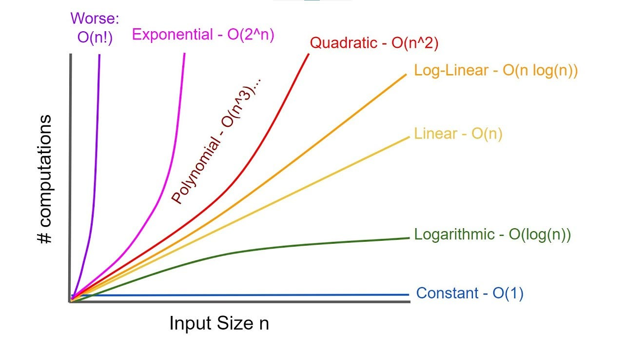
Having a look an a “simple” operation, and how it scale with input:

Of course! Here is the completed markdown table.

A crucial assumption made in these calculations is that a single computation takes approximately 1 nanosecond ( $1 0^{- 9}$ seconds). In reality, this can vary, but it’s a reasonable starting point for illustration.

Count	$O (1)$	$O (lo g (n))$	$O (N)$	$O (N lo g (N))$	$O (N^{2})$	$O (2^{n})$	$O (N!)$
1	1 ns	0 ns	1 ns	0 ns	1 ns	2 ns	1 ns
10	1 ns	3 ns	10 ns	33 ns	100 ns	1.02 µs	3.63 ms
20	1 ns	4 ns	20 ns	86 ns	400 ns	1.05 ms	77.1 years
50	1 ns	6 ns	50 ns	282 ns	2.5 µs	35.7 years	> Age of Universe
100	1 ns	7 ns	100 ns	664 ns	10 µs	> Age of Universe	> Age of Universe
1,000	1 ns	10 ns	1 µs	9.96 µs	1 ms	> Age of Universe	> Age of Universe
10,000	1 ns	13 ns	10 µs	133 µs	100 ms	> Age of Universe	> Age of Universe
100,000	1 ns	17 ns	100 µs	1.66 ms	10 s	> Age of Universe	> Age of Universe
1,000,000	1 ns	20 ns	1 ms	19.93 ms	16.67 min	> Age of Universe	> Age of Universe

Formal Definition of Complexity

We define complexity formally using the Asymptotic Order of Growth. This is a mathematical way to describe how a function behaves as its input grows towards infinity.

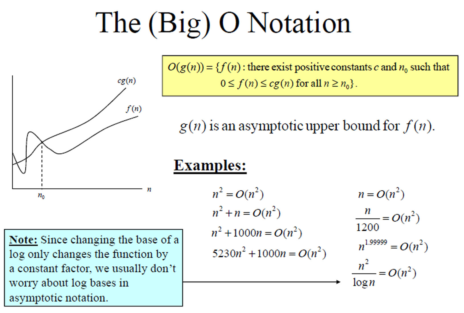
Upper Bound - Big O Notation

T (n) = O (f (n)) if there exist positive constants c and n_{0} such that T (n) \leq c \cdot f (n) for all n \geq n_{0}

This means that for sufficiently large input sizes, the function $T (n)$ does not grow faster than a constant multiple of $f (n)$ .

Lower Bound - Omega Notation

T (n) = Ω (f (n)) if there exist positive constants c and n_{0} such that T (n) \geq c \cdot f (n) for all n \geq n_{0}

Likewise, this means that for sufficiently large input sizes, the function $T (n)$ does not grow slower than a constant multiple of $f (n)$ .

Tight Bound - Theta Notation

T (n) = Θ (f (n)) if there exist positive constants c_{1}, c_{2}, and n_{0} such that c_{1} \cdot f (n) \leq T (n) \leq c_{2} \cdot f (n) for all n \geq n_{0}

And finally, this means that for sufficiently large input sizes, the function $T (n)$ grows at the same rate as a constant multiple of $f (n)$ .

The intuition behind these notations is to provide a way to classify algorithms based on their efficiency and scalability. By understanding the growth rates of different functions, we can make informed decisions about which algorithms to use for specific problems, especially as the size of the input data increases.

Properties of Complexity

Along with the definitions, there are some useful properties of complexity that can help in analyzing algorithms:

Transitivity

If f (n) = O (g (n)) and g (n) = O (h (n)), then f (n) = O (h (n))

This means that if one function is bounded above by a second function, and the second function is bounded above by a third function, then the first function is also bounded above by the third function.

If f (n) = Ω (g (n)) and g (n) = Ω (h (n)), then f (n) = Ω (h (n))

This means that if one function is bounded below by a second function, and the second function is bounded below by a third function, then the first function is also bounded below by the third function.

If f (n) = Θ (g (n)) and g (n) = Θ (h (n)), then f (n) = Θ (h (n))

This means that if one function is tightly bounded by a second function, and the second function is tightly bounded by a third function, then the first function is also tightly bounded by the third function.

Additivity

If f (n) = O (h (n)) and g (n) = O (h (n)), then f (n) + g (n) = O (h (n))

This means that if two functions are both bounded above by a third function, then their sum is also bounded above by that third function.

If f (n) = Ω (h (n)) and g (n) = Ω (h (n)), then f (n) + g (n) = Ω (h (n))

This means that if two functions are both bounded below by a third function, then their sum is also bounded below by that third function.

If f (n) = Θ (h (n)) and g (n) = Θ (h (n)), then f (n) + g (n) = Θ (h (n))

This means that if two functions are both tightly bounded by a third function, then their sum is also tightly bounded by that third function.

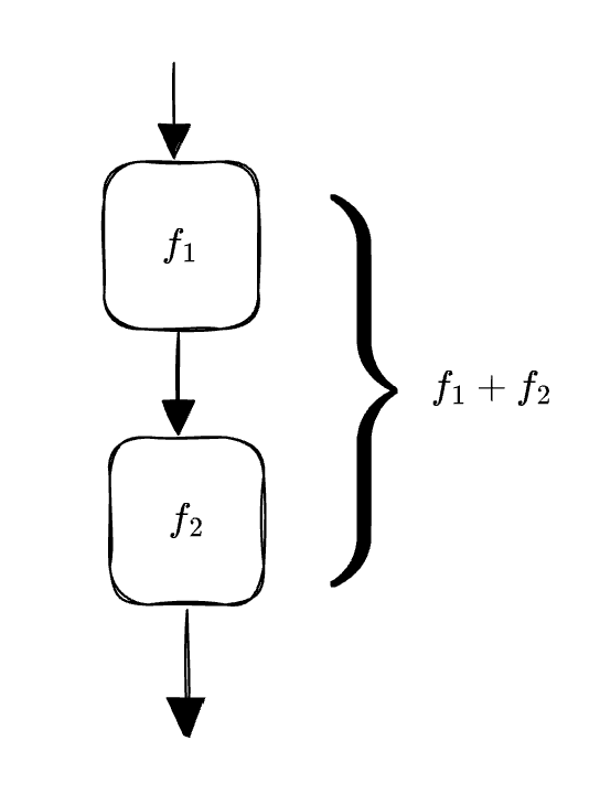
As seen above, the law of additivity can be visualized as stringing together two functions. The overall growth rate is determined by the faster-growing function.

Common Examples of Asymptotic Bounds

To make this process simpler, we can illustrate the values for some general cases of complexity.

Polynomials

a_{0} + a_{1} n + \dots + a_{d} n^{d} is Ω (n^{d}) if a_{d} > 0

Polynomials are bounded below by their highest degree term. This means that as $n$ grows large, the term with the highest degree dominates the growth of the polynomial.

Constant Factor

O (f (n)) = O (c f (n))

Constant factors do not affect the asymptotic growth rate of a function. This means that multiplying a function by a constant does not change its Big O classification.

Logarithms

O (lo g_{a} n) = O (lo g_{b} n) for any constants a, b > 0

Logarithms with different bases are asymptotically equivalent. This means that the base of the logarithm does not affect its growth rate.

For every x > 0, lo g n = O (n^{x})

Logarithms grow slower than any polynomial. This means that as $n$ grows large, logarithmic functions increase at a much slower rate compared to polynomial functions.

Exponentials

For every r > 1 and every d > 0, n^{d} = O (r^{n})

Exponential functions grow faster than any polynomial. This means that as $n$ grows large, exponential functions increase at a much faster rate compared to polynomial functions.

Graph View