Homework 2 - Linear First-Order Equations

Quiz 1 Practice · Lecture 2 - Linear First-Order Differential Equations · Homework 1

Assigned order from the course website. Problem statements are condensed from the textbook scans; numbering and mathematical data are retained.

Obtain solutions using the class methods. For homogeneous equations, first check whether Lecture 2’s exponential or power-law form applies. Computer algebra is a check, not the derivation.

Section 2.1

Classify each equation as linear or nonlinear. For linear equations, also identify homogeneous or nonhomogeneous. Keep any restrictions from denominators when rearranging.

Problem	Equation
1	$y^{\prime }-\sin t=t^{2}y$
3	$\frac{y^{\prime }}{y}-y\cos t=t$
5	$y^{\prime }\sin t=\frac{t^2+1}{y}$
6	$2ty+e^t{y}^{\prime }=\frac{y}{t^2+4}$
9	$\frac{t{y}^{\prime }}{(t^4+2)y}=\cos t+\frac{e^{3t}}{y}$

Section 2.2

For 1, 3, 4, 7, find the general solution, then impose the initial condition.

Problem	IVP
1	$y^{\prime }+3y=0,y(0)=-3$
3	$2ty-y^{\prime }=0,y(1)=3$
4	$t{y}^{\prime }-4y=0,y(1)=1$
7	$2y^{\prime }+3y=e^t,y(0)=0$

For 11, 14, 20, 21, find the general solution.

Problem	Equation
11	$t{y}^{\prime }+4y=0$
14	$(t^2+1)y^{\prime }+2ty=0$
20	$y^{\prime }+2ty=t$
21	$t{y}^{\prime }+2y=t^2,t>0$

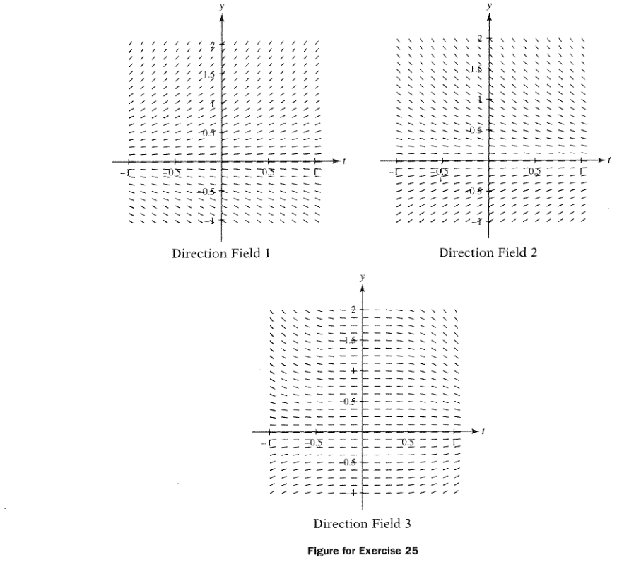
25

Match the equations to direction fields 1–3.

$$\text{(a) }{y}^{\prime }+y=0,\text{(b) }{y}^{\prime }+t^{2}y=0,\text{(c) }{y}^{\prime }-y=0.$$

27

The solution of $t{y}^{\prime }-\alpha y=0$, $y(1)=y_0$ passes through $(2,1)$ and $(4,4)$. Find $\alpha ,y_0$.

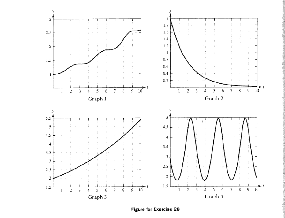
28

Match equations (a)–(d) with graphs 1–4 and recover $y(0)$ for each.

$$\begin{array}{rl}\text{(a)}& 2y^{\prime }+y=0,\\ \text{(b)}& y^{\prime }+(\cos 2t)y=0,\\ \text{(c)}& 10y^{\prime }-(1-\cos 2t)y=0,\\ \text{(d)}& 10y^{\prime }-y=0.\end{array}$$

Instructor hint

Examine the sign of $y^{\prime }$ and what it says about increasing or decreasing $y$. Compare with the exponential-growth discussion in Lecture 2.

36

Solve and determine whether a finite limit exists as $t\to \infty$:

$$y^{\prime }+y+y\cos t=1+\cos t,y(0)=3.$$

Instructor hint

Solve the IVP first. The relation between $g(t)$ and $p(t)$ makes the integrating-factor integral a substitution integral.

37

Solve and determine the long-term behavior:

$$\frac{y^{\prime }-e^{-t}+2}{y}=-2,y(0)=-2.$$

Instructor hint

Solve first, then use the behavior of exponentials as $t\to \infty$. The displayed equation requires $y\ne 0$.

39

For a nonconstant solution of $y^{\prime }+\lambda y=1$, determine which real $\lambda$ give a finite limit as $t\to \infty$, and find that limit.

Instructor hint

Use the constant-coefficient, constant-forcing solution from Lecture 2.

29(c)

Antioxidant activity obeys

$$\frac{dA}{dc}=k(A^{\ast }-A),A(0)=0,k>0,A^{\ast }>0.$$

Find the concentration $c$ at which $A(c)=0.95A^{\ast }$, as a function of $k$.

Instructor hint

Use the solution obtained by shifting to equilibrium in Lecture 2, topic 5; this supplies the earlier parts of the textbook problem.

41

Find a continuous solution on $[0,2\pi ]$:

$$y^{\prime }+(\sin t)y=g(t),y(0)=3,g(t)=\{\begin{array}{ll}\sin t,& 0\le t\le \pi ,\\ -\sin t,& \pi <t\le 2\pi .\end{array}$$

Assigned reading method

Solve on the first interval, evaluate the solution at $\pi$, and use that value as the initial condition on the second interval. This is the method in the assigned textbook reading, pp. 25–26. See Lecture 2 - Linear First-Order Differential Equations > Piecewise coefficients.

Section 2.3

For each cooling curve, determine the initial temperature and the constant temperature of the surroundings.

Problem	Temperature
19	$\theta (t)=70+270e^{-t}{}^{\circ }\mathrm{F}$
21	$\theta (t)=80-40e^{-2t}{}^{\circ }\mathrm{F}$

Use Newton’s cooling law from Lecture 1 and the equilibrium shift from Lecture 2.

Section 2.9

18(a,b)

A 180-lb skydiver drops from rest. After 10 s of free fall, a parachute opens; the skydiver lands 4 s later. Neglect drag before opening, then use drag proportional to velocity. The same parachute gives a 200-lb person terminal velocity $-10$ mph, with upward positive.

Find (a) the speed immediately before opening and (b) the impact velocity.

Instructor guidance

Read pp. 78–79, linear drag only. Use $v^{\prime }=-g-(k/m)v$ and Lecture 2’s constant-shift solution. Mass enters through $k/m$. You may use $g=9.8m/{\mathrm{s}}^2$; first convert mph to m/s. Reset the clock at opening, using the free-fall velocity as the new initial value.

Sources and answer checks

Assignment and instructor hints, checked September 9, 2026.

Textbook: Kohler and Johnson, Elementary Differential Equations, 2nd ed. Local scans: MATH3230-HW-sec2.1-2.4.pdf (assigned exercises on printed pp. 17–18, 26–29, 41), MATH3230-HW-sec2.2-pp25-26.pdf (piecewise method), MATH3230-HW-sec2.9.pdf (linear-drag reading on pp. 78–79; exercise on p. 87).

Posted answers: MATH3230-HW-answers-sec2.1-2.4.pdf. The optional extra-credit problems are separate from this regular assignment.