Markov Chains Explained - 1

for a Normalized Nerd video

Markov chains are used for everything - statistics, biology, and machine learning of course. They allow for some very interesting probability theory.

Let’s start with an example.

---

Imagine there is a restaurant that serves 3 different kinds of foods: burger, pizza, and hot-dog. However, they have a weird rule where they only serve one of these 3 items on any given day. And, it depends on what they served yesterday.

Essentially, if you know the probabilities and what they served today, you could predict what they will serve tomorrow.

Let’s say we are given a graph with all 3 foods, with arrows pointing to other foods with a number between 0 and 1 for their probability.

If we are on pizza today, we can predict that there is a $70\%$ chance of having hotdogs tomorrow.

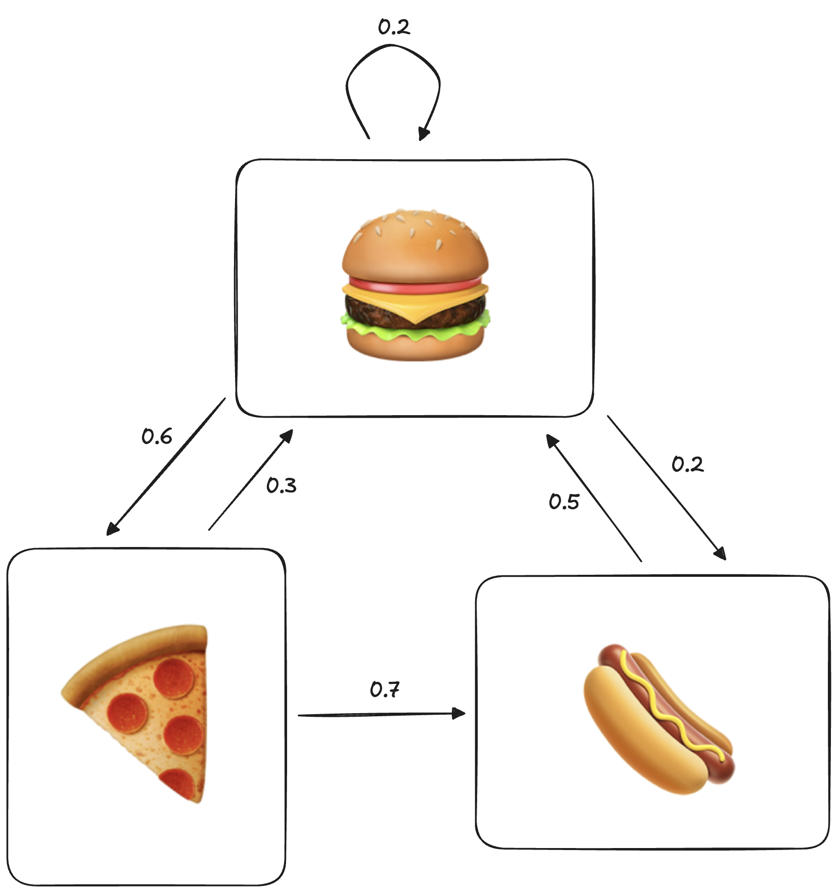
While quite a simple diagram, this is actually a complete Markov chain!

In more formal math notation, we can represent the probability of a certain food choice on a given day considering only what was had yesterday:

$$P(X_{n+1}=x|X_1=x_1,X_2=x_2,\dots ,X_n=x_n)$$

This is the essential property of Markov chains: you only need the previous state to figure out the next, and not the whole history/probability distribution.

Example

For finding the probability of getting Hotdog given that the previous day had Pizza(on the $4_{th}$ day):

$$P(X_4=HOTDOG|X_3=PIZZA)=0.7$$

This is known as the Markov Property.

The other important property is that sum of the weights of the outgoing arrows from any state is equal to 1. This makes sense, as 1 represents the total probability of an action, and if all options dont add up to it, something is wrong.

However, there are special Markov Chains with unique properties that break this rule, we will discuss later.

---

Exploring the Probability Distribution

To get a feel for what you might see over a long time period of this chain, lets walk the chain and see what we get:

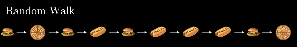
After 10 steps, we are left with this. But how can we find the probability of each of the food items, aka a probability distribution? This is not a particularly meaningful question as it is quite simple, but leads to a bigger picture idea later.

Well, for each food we get the number of occurrences over the total sample size.

$$\begin{array}{rl}P(PIZZA)& =\frac{2}{10}\\ P(BURGER)& =\frac{4}{10}\\ P(HOTDOG)& =\frac{4}{10}\end{array}$$

The more interesting question though, is what do these probabilities converge to? Aka, how does this new Markov graph translate to our more traditional probability summarization methods?

Let’s approach this with a brute force python implementation:

Python

import random # verbose, but clear transitions = { "burger": [ ("burger", 0.2), ("pizza", 0.6), ("hotdog", 0.2) ], "pizza": [ ("burger", 0.3), ("hotdog", 0.7) ], "hotdog": [ ("hotdog", 0.5), ("burger", 0.5) ], } counts = {"burger": 0, "pizza": 0, "hotdog": 0} # initial state state = "burger" # approximation value, kind of like a derivative step dx steps = 100000 for _ in range(steps): # update counts counts[state] += 1 # gets transistions for a state, extracts keys and values options, probs = zip(*transitions[state]) state = random.choices(options, probs)[0] # convert counts to probabilities total = sum(counts.values()) estimated_probs = {k: v / total for k, v in counts.items()} print("Estimated probabilities after simulation:") for food, prob in estimated_probs.items(): print(f"{food}: {prob:.4f}")

Output

Running this, we find that the items converge to some interesting and quite specific values.

$$\begin{array}{r}P(burger):0.3521\\ P(pizza):0.2112\\ P(hotdog):0.4366\end{array}$$

After this point, the distribution reaches a stationary state meaning it will no longer change with time. While this works, this is not a very efficient way to compute the distribution, and leaves the question if there is a more mathematical approach. We also dont know if there are any other stationary states.

Well, there is a better way to represent it, through the user of Linear Algebra

---

Using Matrices for Markov Representations

In reality, a Markov change is essentially just a directed graph, something we are very familiar with (as computer scientists for graph databases, and in theory of computing with Automota)

Because of this, we can represent the previous graph with a simple adjacency matrix:

$$\begin{array}{cccc}\text{From}\backslash \text{To}& \text{Burger}& \text{Pizza}& \text{Hotdog}\\ \text{Burger}& 0.2& 0.6& 0.2\\ \text{Pizza}& 0.3& 0& 0.7\\ \text{Hotdog}& 0.5& 0.5& 0\end{array}$$

Where the Columns represent the initial state, and the Rows represent the destination state.

In Linear Algebra, we would represent this as a Transition Matrix $A$:

$$A=\left[\begin{array}{ccc}0.2& 0.6& 0.2\\ 0.3& 0& 0.7\\ 0.5& 0& 0.5\end{array}\right]$$

We will then use a secondary matrix $\pi$ to represent the probability distribution of the states. As the Markov Chain progresses through time, the matrix will approach values like the ones we found with the python Approach.

If we begin on a pizza day, the first state of the $\pi$ matrix would look like:

$${\pi }_0=\left[\begin{array}{ccc}0& 1& 0\end{array}\right]$$

Something interesting happens when we multiply these two matrices together:

$${\pi }_{0}A=\left[\begin{array}{ccc}0& 1& 0\end{array}\right]\left[\begin{array}{ccc}0.2& 0.6& 0.2\\ 0.3& 0& 0.7\\ 0.5& 0& 0.5\end{array}\right]=\left[\begin{array}{ccc}0.3& 0& 0.7\end{array}\right]$$

We have extracted the second row of the transition matrix, which happens to represent the probabilities of future foods given it is a pizza day.

Now, if you take this resulting value and put it in the place of the initial ${\pi }_0$ matrix:

$${\pi }_{1}A=\left[\begin{array}{ccc}0.3& 0& 0.7\end{array}\right]\left[\begin{array}{ccc}0.2& 0.6& 0.2\\ 0.3& 0& 0.7\\ 0.5& 0& 0.5\end{array}\right]=\left[\begin{array}{ccc}0.41& 0.18& 0.41\end{array}\right]$$

We get this new interesting value. What does it mean? Let’s repeat this a few more time for the next few iterations of $\pi$:

$${\pi }_{2}A=\left[\begin{array}{ccc}0.41& 0.18& 0.41\end{array}\right]\left[\begin{array}{ccc}0.2& 0.6& 0.2\\ 0.3& 0& 0.7\\ 0.5& 0& 0.5\end{array}\right]=\left[\begin{array}{ccc}0.34& 0.25& 0.41\end{array}\right]$$

Notice how this seems to be getting closer and closer to the stationary state? Thats because it is!

If there exists a stationary state for this initial choice, then after repeating the process several times, the resultant matrix will converge on a stationary value. Eventually, the output vector will be identical to the input vector.

Denoting this special row vector as $\pi$ we can write(for a converging stationary state):

$$\pi A=\pi$$

As Linear Algebra students, we will recognize this as similar to the eigenvector equation:

$$Av=\lambda v$$

Just by considering $\lambda =1$ and reversing the order of multiplication, we get our equilibrium state equation.

How do we interpret this? We imagine $\pi$ is a left eigenvector of matrix $A$, with the eigenvalue equal to 1.

The eigenvector in this approach must also satisfy another condition: the elements of $\pi$ must add up to 1( as it is a probability distribution ).

$$\pi [1]+\pi [2]+\pi [3]=1$$

After solving these two equation, we are left with the finalized stationary state:

$$\pi =\left[\begin{array}{ccc}\frac{25}{71}& \frac{15}{71}& \frac{31}{71}\end{array}\right]$$

Converting to decimal:

$$\pi =\left[\begin{array}{ccc}0.35211& 0.21127& 0.43662\end{array}\right]$$

Very similar to our brute force approach!

Using this technique, we can also find out if there are more than one stationary state. This can be done, as you might expect, by finding out if there exists any more than one eigenvectors! Very nice.