The most basic of the ODE approximation methods, Euler’s Method is a first-order numerical procedure for solving ordinary differential equations (ODEs) with a given initial value.
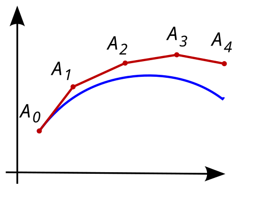
The essential idea is to use the slope of the function at a known point to estimate the value of the function at the next point. E.g., you calculate the slope, take a step in that direction, and repeat. This is actually pretty accurate for small steps, but the error accumulates quickly over larger intervals. A good example of it blowing up is with sine waves/spring predication, the errors compounds and the wave amplitude blows up out of control.
A general formula for RK1 Eulers Method could look like:
Implicit Vs Explicit
Explicit Euler Method takes a sample at the current point and uses that to estimate the next point. This has the opposite problem of the sine wave example, where the amplitude blows up.
The same thing happens but with amplitude decay, the amplitude decays too quickly and the wave flattens out.
However, there is also the implicit Euler method, which is more stable for stiff equations. In this version, you use the slope at the next point to estimate the value of the function, which requires solving an equation at each step but can handle larger steps without becoming unstable.
How to Fix This?
The solution is something called the Runge Kutta, which is a more sophisticated method that takes multiple samples within each step to get a better estimate of the slope. The most common version is the fourth-order Runge-Kutta method (RK4), which averages slopes at several points within the interval to achieve much higher accuracy.