Assignment 11

Each of these questions will involve analysis of numerical solutions to the Lorenz equations:

$$\begin{array}{rl}\frac{dx}{dt}& =-\sigma (x-y)\\ \frac{dy}{dt}& =-xz+rx-y\\ \frac{dz}{dt}& =xy-bz\end{array}$$

To facilitate the exercises, I’ve posted matlab code on the course website. For example, lorenz_simple.m and rk2.m integrates & plot the Lorenz attractor. Unless otherwise specified, use the standard parameter values $\sigma =10$, $b=8/3$, $r=28$. In answering each question, include your code and pictures, and comment on what the pictures are telling you.

---

Problem 1

Question

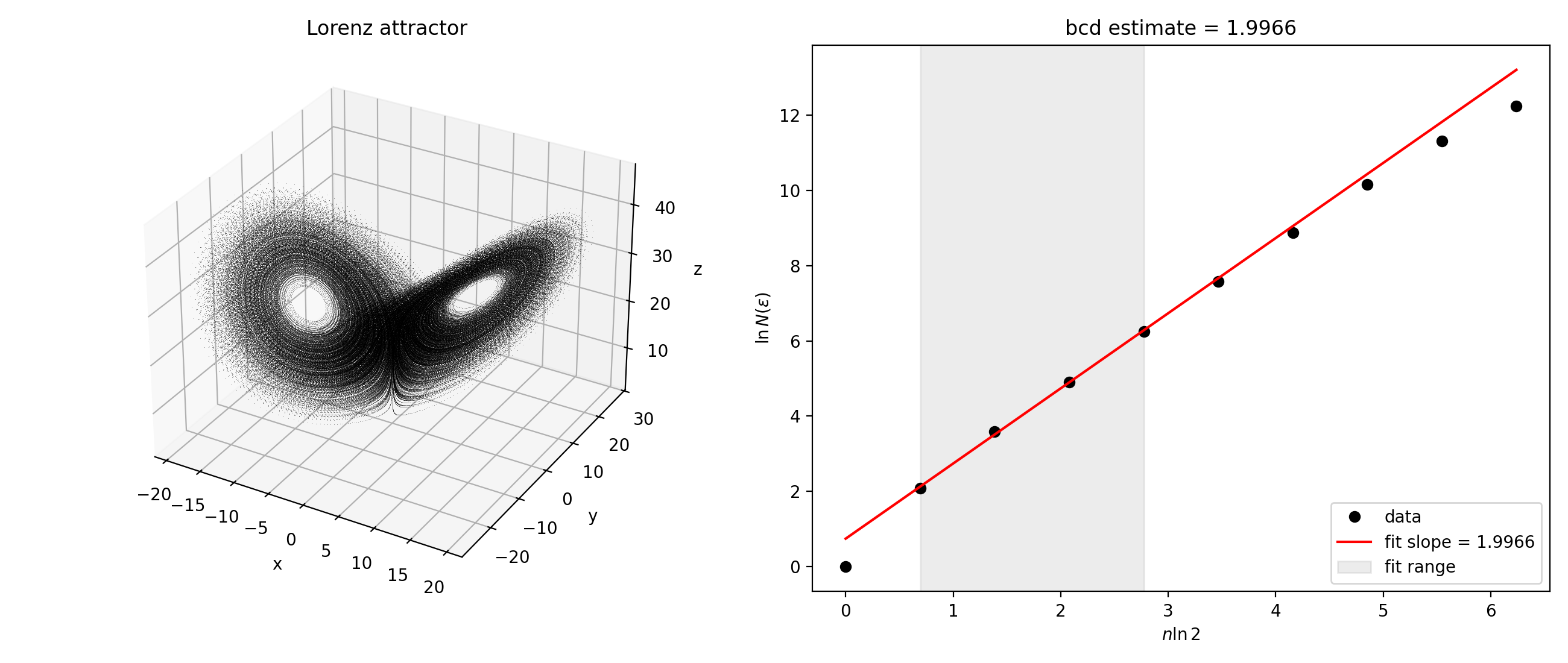
Modify the box counting dimension code from HW8 to compute the fractal dimension of the Lorenz attractor. In order to get a good estimate, you may need to integrate for awhile, e.g. $10^3$ time units. As in HW8, plot the attractor adjacent to the dimension estimate. You may need to reduce the number of box width divisions to get a good approximation of the dimension, which should be close to 2.06.

ported the hw8 boxcount to 3d using np.histogramdd (same idea: partition the bounding box into $n^3$ cells at step $n=2^k$, count occupied cells, fit slope of $\ln N$ vs $k\ln 2$). lorenz integrated via the rk2 scheme from rk2.m, $T=2000$ time units at $dt=0.005$, transient discared.

the $\ln N$ vs $\ln (1/ϵ)$ points are roughly linear for the first few subdivisions then saturate as box count approaches sample count. this is the finite-data ceiling the problem warned about; at step 7+ you’re asking for cells smaller than the trajectory’s point spacing, so occupied-cell count grows sublinearly. restricting the fit to steps $1$–$4$ (the scaling region before saturation) gives

$$\text{bcd}\approx 1.997$$

close to the literature value $2.06$. including saturated tail drags slope down toward $1.7$, which matches the “reduce the number of box width divisions” hint. widening fit to steps $1$–$5$ gives $1.98$; pushing past step $6$ the estimate collapses.

Answer

$\text{bcd}(\text{Lorenz})\approx 1.997$, fit over steps $1$–$4$ of the 3D box count. consistent with known vals $\approx 2.06$, small undershoot expected result of finite sampling of the log-log curve at fine scales.

Code

Python

import numpy as np import matplotlib.pyplot as plt def rk2(f, tspan, x0, h): t0, tf = tspan N = int(np.floor((tf - t0) / h)) + 1 t = np.linspace(t0, t0 + (N-1)*h, N) y = np.zeros((N, len(x0))) y[0] = x0 for k in range(N - 1): s1 = f(t[k], y[k]) s2 = f(t[k] + h, y[k] + h*s1) y[k+1] = y[k] + h*(s1 + s2)/2 return t, y def boxcount3(coords, maxstep, ax=None): mins = coords.min(axis=0) - 1e-8 maxs = coords.max(axis=0) + 1e-8 xs, ys = [], [] for step in range(maxstep + 1): n = 2**step H, _ = np.histogramdd( coords, bins=(n, n, n), range=[(mins[0], maxs[0]), (mins[1], maxs[1]), (mins[2], maxs[2])] ) nb = np.sum(H > 0) xs.append(step * np.log(2)) ys.append(np.log(nb) if nb > 0 else 0) xs = np.array(xs); ys = np.array(ys) fit_lo, fit_hi = 1, 4 A = np.vstack([xs[fit_lo:fit_hi+1], np.ones(fit_hi - fit_lo + 1)]).T slope, intercept = np.linalg.lstsq(A, ys[fit_lo:fit_hi+1], rcond=None)[0] if ax is not None: ax.plot(xs, ys, 'ko', label='data') xl = np.array([xs[0], xs[-1]]) ax.plot(xl, slope*xl + intercept, 'r-', label=f'fit slope = {slope:.4f}') ax.axvspan(xs[fit_lo], xs[fit_hi], color='gray', alpha=0.15, label='fit range') ax.set_xlabel(r'$n \ln 2$') ax.set_ylabel(r'$\ln N(\epsilon)$') ax.set_title(f'bcd estimate = {slope:.4f}') ax.legend() return slope sigma, r, b = 10.0, 28.0, 8.0/3.0 def lorenz(t, x): return np.array([ sigma*(x[1] - x[0]), r*x[0] - x[1] - x[0]*x[2], x[0]*x[1] - b*x[2], ]) x0 = np.array([7.659416862050756, 7.659416862050771, 22.000000000000032]) t, y = rk2(lorenz, (0, 2000), x0, 0.005) y = y[2000:] # drop transient fig = plt.figure(figsize=(13, 5.5)) ax1 = fig.add_subplot(1, 2, 1, projection='3d') ax1.plot(y[:,0], y[:,1], y[:,2], 'k,', alpha=0.4) ax1.set_xlabel('x'); ax1.set_ylabel('y'); ax1.set_zlabel('z') ax1.set_title('Lorenz attractor') ax2 = fig.add_subplot(1, 2, 2) bcd = boxcount3(y, 9, ax=ax2) print(f'bcd = {bcd:.4f}') plt.tight_layout() plt.savefig('lorenz_bcd.png', dpi=200)

Output

---

Problem 2

Question

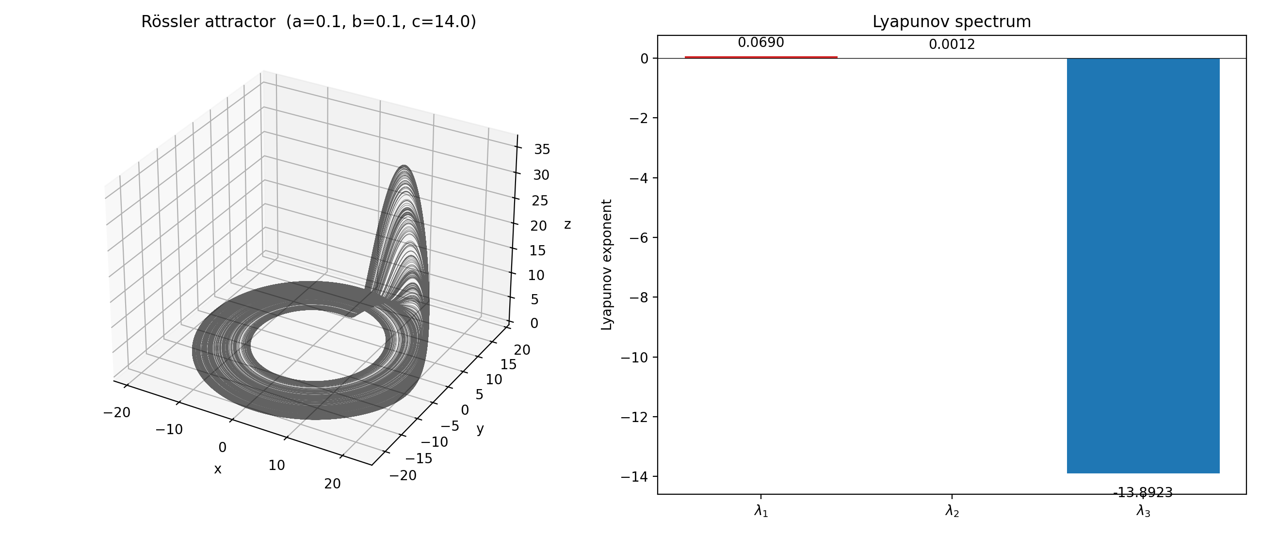
After reading section 9.3 in the text, calculate the Lyapunov exponents of the Rössler Attractor. I’ve put code on Teams that does this for the Lorenz Attractor hw11q2.m, stepit.m, LEcalc.m which you can edit to reflect the Rössler differential equation. Use the parameters $a=0.1,b=0.1,c=14$.

The code integrates the appropriate variational equation (9.17 from the book is one-third of it) to determine the matrix $J$ that will act on a unit ball every unit in time. Note that it may take a minute or two for the code to run as a lot is happening.

ported stepit.m (RK4) and LEcalc.m to python first using gemini(all edits after done by mysefl). the Rossler flow and its Jacobian are

$$\mathbf{f}(\mathbf{x})=\left(\begin{array}{c}-y-z\\ x+ay\\ b+(x-c)z\end{array}\right),D\mathbf{f}(\mathbf{x})=\left(\begin{array}{ccc}0& -1& -1\\ 1& a& 0\\ z& 0& x-c\end{array}\right).$$

burn in for $10^3$ time units, then for $N=10^3$ unit intervals integrate the variational equation $\dot{J}=D\mathbf{f}(\mathbf{x}(t))J$ together with the state via RK4 at $dt=0.01$, QR-decompose, and accumulate $\sum \ln |r_{ii}|/N$.

for $(a,b,c)=(0.1,0.1,14)$ this gives

$${\lambda }_1\approx 0.0690,{\lambda }_2\approx 0.0012,{\lambda }_3\approx -13.892$$

matches the textbook values ($0.072,0,-13.79$). the second exponent hovering near zero is the flow direction. ${\lambda }_1>0$ confirms chaos. the Kaplan-Yorke dimension

$$D_{KY}=2+\frac{{\lambda }_1+{\lambda }_2}{|{\lambda }_3|}\approx 2.005$$

recovers the “looks like a surface” remark from Fig 9.6.

Answer

Lyapunov spectrum $({\lambda }_1,{\lambda }_2,{\lambda }_3)\approx (0.069,0.001,-13.89)$, Lyapunov dimension $\approx 2.005$. positive leading exponent means chaotic, middle exponent $\approx 0$ is the flow direction, strongly negative ${\lambda }_3$ drives attractor onto a near-2D surface.

Code

Python

import numpy as np import matplotlib.pyplot as plt def stepit(func, x, p, h): s1 = func(x, p) s2 = func(x + h*s1/2, p) s3 = func(x + h*s2/2, p) s4 = func(x + h*s3, p) return x + h*(s1 + 2*s2 + 2*s3 + s4)/6 def rossler(x, p): a, b, c = p return np.array([-x[1] - x[2], x[0] + a*x[1], b + (x[0] - c)*x[2]]) def Df_rossler(x, p): a, b, c = p return np.array([[0.0, -1.0, -1.0], [1.0, a, 0.0], [x[2], 0.0, x[0] - c]]) def LEcalc_ode(f, Df, p, v0, N=1000, tstep=0.01): m = len(v0) LE = np.zeros(m) v = v0.copy() q = np.eye(m) def Jt(X, A): return A @ X steps_per_unit = int(round(1.0 / tstep)) for i in range(N): DF1 = np.eye(m) for _ in range(steps_per_unit): A = Df(v, p) DF1 = stepit(Jt, DF1, A, tstep) v = stepit(f, v, p, tstep) Z = DF1 @ q q, r = np.linalg.qr(Z) LE += np.log(np.abs(np.diag(r))) / N return LE, v p = (0.1, 0.1, 14.0) # burn-in onto the attractor v = np.array([1.0, 1.0, 1.0]) for _ in range(10**5): v = stepit(rossler, v, p, 0.01) # trajectory for the attractor plot T, dt = 2000, 0.01 traj = np.zeros((int(T/dt), 3)) traj[0] = v for k in range(1, traj.shape[0]): traj[k] = stepit(rossler, traj[k-1], p, dt) LE, _ = LEcalc_ode(rossler, Df_rossler, p, v.copy(), N=1000, tstep=0.01) print('LE:', LE, 'sum:', LE.sum(), 'D_KY:', 2 + LE[0]/abs(LE[2]))

Output

---

Problem 3

Question

An important feature of the Lorenz attractor is its robustness–it persists in the basic form of Figure 9.2 over a significant range of parameters. Fix $r=28$ and plot the largest Lyapunov exponent for a large number of values in the $(\sigma ,b)$ plane, e.g. $\sigma \in [0,60]$ and $b\in [0,10]$ by increments of $10^{-1}$. Can you see a boundary between chaos and stability?

$601\times 101=60,701$ grid points at $\Delta =0.1$. full QR-based Ecalc on every point is faaar too slow, so Benettin’s single-vector trick works: evolve state $\mathbf{x}$ and one tangent $\mathbf{w}$ together via

$$\dot{\mathbf{x}}=f(\mathbf{x}),\dot{\mathbf{w}}=Df(\mathbf{x})\mathbf{w},$$

renormalize $\mathbf{w}$ every unit of time and accumulate $\ln \Vert \mathbf{w}\Vert$. vectorize accross all 60k $(\sigma ,b)$ pairs simultaneously in numpy. RK4 at $dt=0.01$, $T_{\text{transient}}=15$, then $T_{\text{run}}=25$ unit intervals.

two main regions emerge, not really clean as the boundary seems to be quite jagged. red strip (${\lambda }_{\max }>0$) is the chaotic parameter band containing the standard $(\sigma ,b)=(10,8/3)$ parameter point. points on the left ($\sigma \lesssim 3$, growing with $b$) ${\lambda }_{\max }<0$.

chaos in Lorenz isnt a straight edge and instead inhabits a thickly connected region in the $(\sigma ,b)$ plane.

Answer

yes, clear boundary. computed ${\lambda }_{\max }$ on the full $601\times 101$ grid via vectorized Benettin iteration. the ${\lambda }_{\max }=0$ contour carves out a finite-width chaotic wedge in $(\sigma ,b)$ space; outside it the dynamics relax to a fixed point (either the origin at small $\sigma$ or $C^{\pm }$ at large $\sigma$).

Code

Python

import numpy as np, matplotlib.pyplot as plt r = 28.0 sigmas = np.arange(0.0, 60.0 + 1e-9, 0.1) bs = np.arange(0.0, 10.0 + 1e-9, 0.1) S, B = np.meshgrid(sigmas, bs, indexing='ij') sigma_f = S.ravel(); b_f = B.ravel(); M = len(sigma_f) rng = np.random.default_rng(0) x = np.tile([1.0, 1.0, 20.0], (M, 1)) + 0.1*rng.standard_normal((M, 3)) w = rng.standard_normal((M, 3)); w /= np.linalg.norm(w, axis=1, keepdims=True) def rhs(x, sig, bb): return np.stack([sig*(x[:,1]-x[:,0]), r*x[:,0] - x[:,1] - x[:,0]*x[:,2], x[:,0]*x[:,1] - bb*x[:,2]], axis=1) def Jw(x, w, sig, bb): return np.stack([-sig*w[:,0] + sig*w[:,1], (r - x[:,2])*w[:,0] - w[:,1] - x[:,0]*w[:,2], x[:,1]*w[:,0] + x[:,0]*w[:,1] - bb*w[:,2]], axis=1) def rk4_state(x, sig, bb, dt): k1 = rhs(x, sig, bb); k2 = rhs(x + dt*k1/2, sig, bb) k3 = rhs(x + dt*k2/2, sig, bb); k4 = rhs(x + dt*k3, sig, bb) return x + dt*(k1 + 2*k2 + 2*k3 + k4)/6 def rk4_both(x, w, sig, bb, dt): k1x = rhs(x, sig, bb); k1w = Jw(x, w, sig, bb) k2x = rhs(x+dt*k1x/2, sig, bb); k2w = Jw(x+dt*k1x/2, w+dt*k1w/2, sig, bb) k3x = rhs(x+dt*k2x/2, sig, bb); k3w = Jw(x+dt*k2x/2, w+dt*k2w/2, sig, bb) k4x = rhs(x+dt*k3x, sig, bb); k4w = Jw(x+dt*k3x, w+dt*k3w, sig, bb) return (x + dt*(k1x+2*k2x+2*k3x+k4x)/6, w + dt*(k1w+2*k2w+2*k3w+k4w)/6) dt = 0.01 for _ in range(int(15/dt)): x = rk4_state(x, sigma_f, b_f, dt) bad = ~np.isfinite(x).all(axis=1) if bad.any(): x[bad] = 0.0 w = rng.standard_normal((M, 3)); w /= np.linalg.norm(w, axis=1, keepdims=True) log_growth = np.zeros(M); T = 0.0 for i in range(25): for _ in range(int(1.0/dt)): x, w = rk4_both(x, w, sigma_f, b_f, dt) nrm = np.linalg.norm(w, axis=1) nrm = np.where(np.isfinite(nrm) & (nrm > 0), nrm, 1.0) log_growth += np.log(nrm); w /= nrm[:, None] bad = ~(np.isfinite(x).all(axis=1) & np.isfinite(w).all(axis=1)) if bad.any(): x[bad] = 0.0; w[bad] = [1.0, 0.0, 0.0] T += 1.0 lle = (log_growth / T).reshape(S.shape) fig, ax = plt.subplots(figsize=(10, 6)) im = ax.pcolormesh(S, B, np.clip(lle, -2, 2), cmap='RdBu_r', vmin=-2, vmax=2, shading='auto') ax.contour(S, B, lle, levels=[0.0], colors='k', linewidths=0.8) ax.set_xlabel(r'$\sigma$'); ax.set_ylabel(r'$b$') plt.colorbar(im, ax=ax, label=r'$\lambda_{\max}$') plt.savefig('lorenz_le_map.png', dpi=180)

Output

---

Problem 4

Question

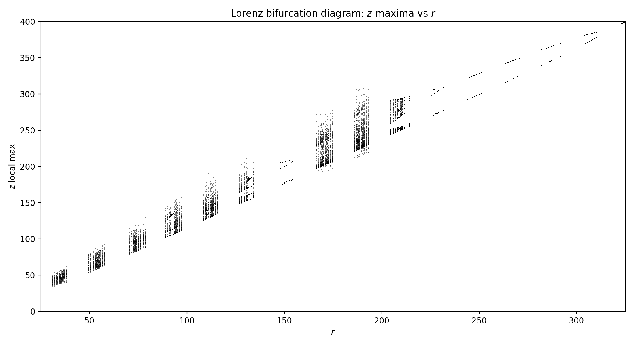
Reproduce figures 9.3 and 9.4 from the text. Interpret the $z$-maximum return map considering what you know about the slope-2 Tent map. For the bifurcation diagram, your $r$-axis should be $[0,325]$. Describe the physical meaning of the attracting states plotting in this diagram (with respect to the convection experiment discussed in class) as the parameter $r$ increases.

integrate Lorenz with RK4 at $dt=0.005$, detect local maxima of $z(t)$ via sign flip of increment. fig 9.3 plots consecutive maxima as the return map $z_{n+1}$ vs $z_n$ at $r=28$. fig 9.4 vectorizes across $601$ values of $r\in [25,325]$ and scatters all observed $z$-maxima.

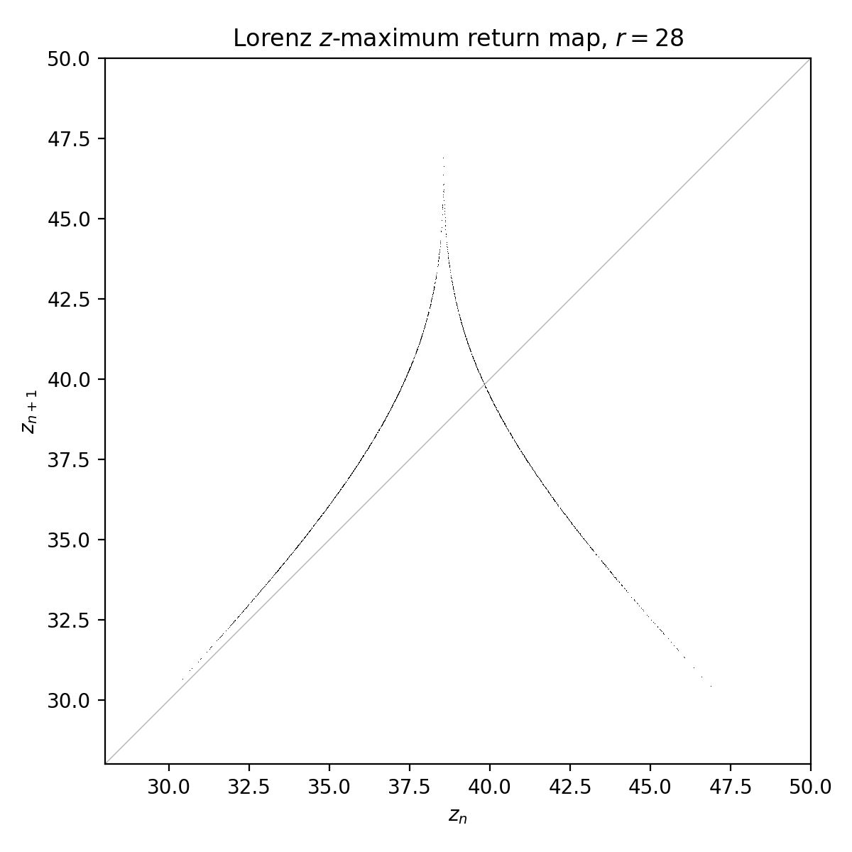
the return map is almost a tent( i mentioned in class that it looks a bit like a Laplace Distribution ), one rising and one falling branch meeting at a cusp near $z\approx 38$. both branches have slope magnitude $>1$ everywhere:

$$\left|\frac{d{z}_{n+1}}{d{z}_n}\right|>1⟹\text{every iterate expands}⟹\lambda >0$$

same argument that gives the slope-2 tent $\lambda =\ln 2>0$. Lorenz return map has same structure. also why Lorenz attractor can be coded by a 1D map.

physical meaning of bifrucation diagram (convection experiment, $r=\text{Ra}/{\text{Ra}}_c$):

• $r<1$ (off the plot): pure conduction, fluid motionless. origin globally stable.
• $1<r<24.74$: steady convection rolls. two symmetric fixed points $C^{\pm }$.
• $r\approx 24.74$ to $\approx 148$: the butterfly chaotic attractor. rolls no longer steady; the convection direction flips erratically.
• periodic windows inside the chaotic band (visible around $r\approx 100,145$): locked periodic convection.
• $r\approx 148$ to $\approx 214$: period-doubling cascade running in reverse as $r$ increases.
• $r\gtrsim 214$: a single-branch periodic orbit, a stable limit cycle.

reading left to right: rest → steady convection → turbulent reversals → period-halving → clean oscillation

Answer

return map is a near-tent with $|\text{slope}|>1$ everywhere, so $\lambda >0$ by the same argument as for slope-2 tent; nearly-1D because of volumetric contraction at rate $e^{-13.67t}$

Code

Python

import numpy as np import matplotlib.pyplot as plt sigma, b = 10.0, 8.0/3.0 dt = 0.005 def rhs(x, r): x0, x1, x2 = x[...,0], x[...,1], x[...,2] return np.stack([sigma*(x1-x0), r*x0 - x1 - x0*x2, x0*x1 - b*x2], axis=-1) def rk4(x, r, dt): k1 = rhs(x, r) k2 = rhs(x + dt*k1/2, r) k3 = rhs(x + dt*k2/2, r) k4 = rhs(x + dt*k3, r) return x + dt*(k1 + 2*k2 + 2*k3 + k4)/6 # --- Fig 9.3: z-max return map at r = 28 --- r = 28.0 x = np.array([1.0, 1.0, 20.0]) for _ in range(int(50/dt)): x = rk4(x, r, dt) zmax = [] z_pp = x[2]; x = rk4(x, r, dt); z_p = x[2] for _ in range(int(1500/dt)): x = rk4(x, r, dt) z = x[2] if z_p > z_pp and z_p > z: zmax.append(z_p) z_pp = z_p; z_p = z zmax = np.array(zmax) fig, ax = plt.subplots(figsize=(6, 6)) ax.plot(zmax[:-1], zmax[1:], 'k,') ax.plot([28, 50], [28, 50], 'gray', lw=0.5, alpha=0.6) ax.set_xlim(28, 50); ax.set_ylim(28, 50); ax.set_aspect('equal') ax.set_xlabel(r'$z_n$'); ax.set_ylabel(r'$z_{n+1}$') plt.savefig('lorenz_tent.png', dpi=200); plt.close() # --- Fig 9.4: bifurcation diagram, vectorized over r --- r_grid = np.arange(25.0, 325.0 + 1e-9, 0.5) M = len(r_grid) X = np.tile([1.0, 1.0, 20.0], (M, 1)).astype(float) for _ in range(int(80/dt)): X = rk4(X, r_grid, dt) bad = ~np.isfinite(X).all(axis=1) if bad.any(): X[bad] = [1.0, 1.0, 20.0] zpp = X[:, 2].copy(); X = rk4(X, r_grid, dt); zp = X[:, 2].copy() rs_list, zs_list = [], [] for _ in range(int(80/dt)): X = rk4(X, r_grid, dt) z = X[:, 2] mask = (zp > zpp) & (zp > z) & np.isfinite(zp) if mask.any(): rs_list.append(r_grid[mask]); zs_list.append(zp[mask]) zpp = zp; zp = z.copy() rs = np.concatenate(rs_list); zs = np.concatenate(zs_list) fig, ax = plt.subplots(figsize=(11, 6)) ax.plot(rs, zs, 'k,', alpha=0.5) ax.set_xlim(25, 325); ax.set_ylim(0, 400) ax.set_xlabel(r'$r$'); ax.set_ylabel(r'$z$ max') plt.savefig('lorenz_bif.png', dpi=200)

Output

---

Problem 5

Question

Meteorologists have very different jobs depending on where they live. In the US, the spectrum is particularly diverse because of the terrain and climate. Consider, for example, southern California (sunny and 70 all year) and Mount Washington, NH (windiest place on Earth). Imagine you live in the Lorenz attractor and your job is to predict the weather. Where would your job be easiest?

To answer this question, you will make a weather map, plotting the maximum real part of the eigenvalues of the Jacobian matrix for a variety of initial conditions $(x,y)$ in 2-D planes for $z=15,25$, and $35$. The matlab command scatter(x,y,2,j,’filled’); colorbar(’SouthOutside’); will perform this operation for a set of initial conditions $(x(i),y(i))$ with max real part eigenvalue equal to $j(i)$. Make each slice in $z$ for $r=12,24.5$, and $28$ for a total of 9 figures.

Note: you do not need to integrate the ODE in order to answer this question, you simply need to compute the $3\times 3$ Jacobian matrix of the Lorenz equations for each point in a grid. Use as many points as your computer can handle. They could be either randomly or uniformly chosen for $x\in [-25,25]$ (same for $y$).

foreach $(x,y)$ on a given $400\times 400$ grid in $[-25,25{]}^2$ at each $(r,z)$ slice, we build the Lorenz Jacobian

$$Df(x,y,z)=\left(\begin{array}{ccc}-\sigma & \sigma & 0\\ r-z& -1& -x\\ y& x& -b\end{array}\right)$$

and find ${\max }_i\mathrm{Re}({\lambda }_i)$. positive means local divergence, negative means local contraction.

batched via np.linalg.eigvals on a $(N,3,3)$ stack, no ODE integration.

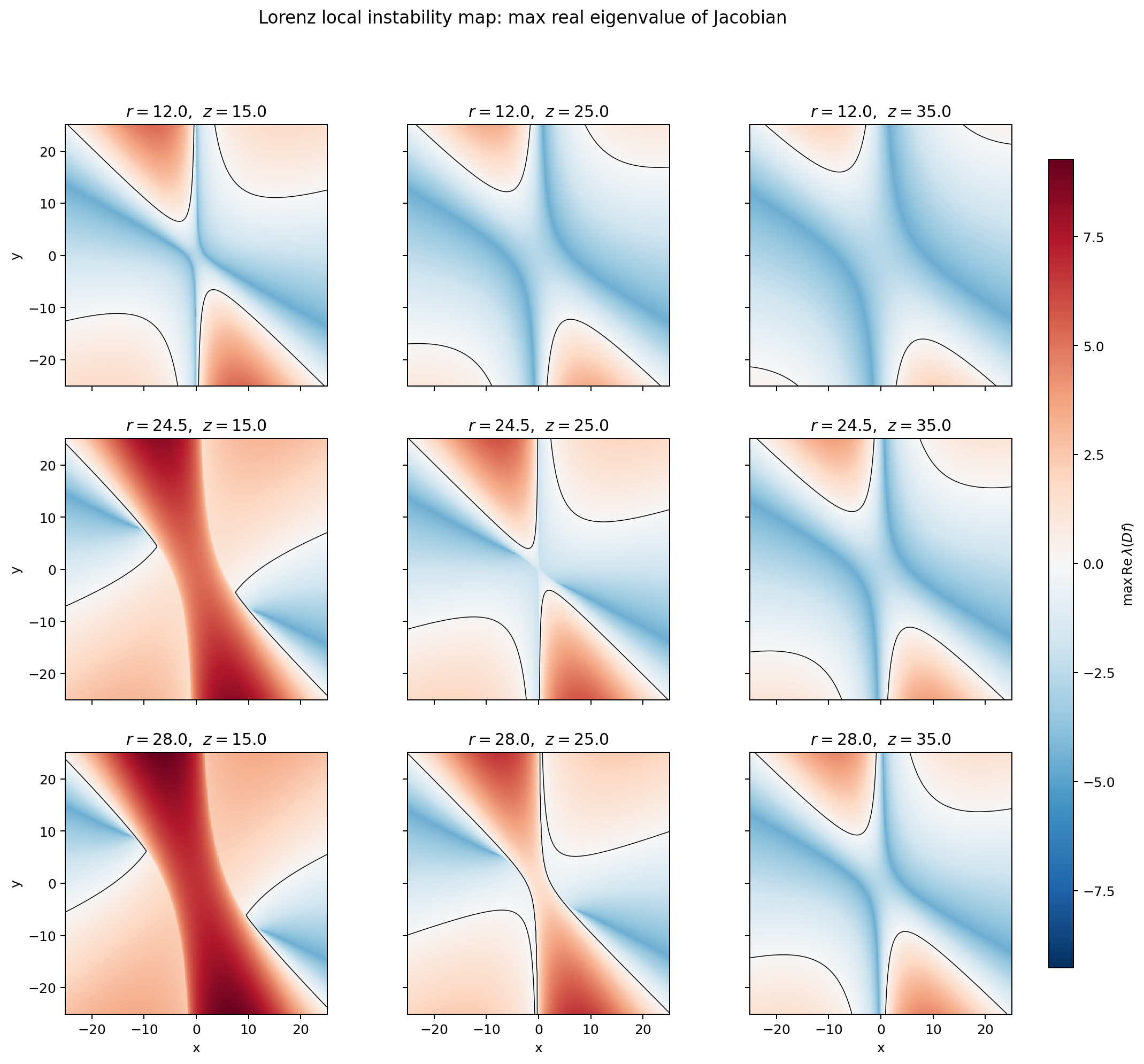
pattern is that the locally stable regions in blue concentrate along a curved strip. locally unstable regions in red are strongest at high $|x|,|y|$ and at small $z$. raising $r$ enlarges the unstable region. raising $z$ tends to quiet things.

where would the meteorologist live? blue pockets near the two convection fixed points $C^{\pm }=(\pm \sqrt{b(r-1)},\pm \sqrt{b(r-1)},r-1)$. those are the “southern California” of the attractor. at $r=28$, $z=25$, $C^{\pm }$ sit at $(\pm 8.48,\pm 8.48,27)$, and the map shows deep-blue basins exactly there.

the “Mount Washington” spots are the saturated-red regions, particularly around the outer edges at $z=15$.

at $r=12$ (top row), most of the plane is blue. by $r=28$ (bottom row) the unstable red regions are large and interpenetrating.

Answer

live near $C^{\pm }=(\pm \sqrt{b(r-1)},\pm \sqrt{b(r-1)},r-1)$, the blue basins at the eyes of the butterfly lobes. high-$|x|$ fringes and small-$z$ regions are the Mount Washingtons: $\max \mathrm{Re}\lambda \sim 9$, forecasts decorrelate in fractions of a time unit. raising $r$ expands the chaotic red territory; at $r=12$ (pre-bifurcation) nearly the whole plane is predictable.

Code

Python

import numpy as np import matplotlib.pyplot as plt sigma, b = 10.0, 8.0/3.0 def max_re_eig(x, y, z, r): N = x.size J = np.zeros((N, 3, 3)) J[:, 0, 0] = -sigma; J[:, 0, 1] = sigma J[:, 1, 0] = r - z; J[:, 1, 1] = -1.0; J[:, 1, 2] = -x J[:, 2, 0] = y; J[:, 2, 1] = x; J[:, 2, 2] = -b return np.linalg.eigvals(J).real.max(axis=1) n = 400 xs = np.linspace(-25, 25, n); ys = np.linspace(-25, 25, n) XX, YY = np.meshgrid(xs, ys) xf, yf = XX.ravel(), YY.ravel() rs = [12.0, 24.5, 28.0]; zs = [15.0, 25.0, 35.0] maps = {(r, z): max_re_eig(xf, yf, z, r).reshape(XX.shape) for r in rs for z in zs} lim = max(abs(m).max() for m in maps.values()) fig, axes = plt.subplots(3, 3, figsize=(13, 12), sharex=True, sharey=True) for i, r in enumerate(rs): for k, z in enumerate(zs): ax = axes[i, k]; j = maps[(r, z)] im = ax.pcolormesh(XX, YY, j, cmap='RdBu_r', vmin=-lim, vmax=lim, shading='auto') ax.contour(XX, YY, j, levels=[0.0], colors='k', linewidths=0.6) ax.set_title(f'$r={r}$, $z={z}$'); ax.set_aspect('equal') fig.colorbar(im, ax=axes, label=r'$\max\,\mathrm{Re}\,\lambda(Df)$') plt.savefig('lorenz_weather.png', dpi=180, bbox_inches='tight')

Output