Stokes' Theorem

We have discussed the orientation of curves and the orientation of surfaces. To state Stoke’s Theorem, we need to discuss boundary orientation:

Sketch

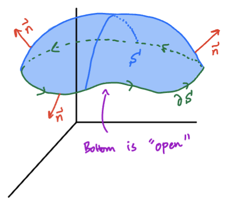
We say $\partial S$ has positive boundary orientation if $S$ is always on your left as you traverse $\partial S$ while standing in the direction of the unit normal vector $n$ .

Remark

The boundary curve can be thought of as where the surface, ends, or the “edge” of a surface. Some surfaces have more than one boundary curve, and closed surfaces have no boundary curve.

Sketch

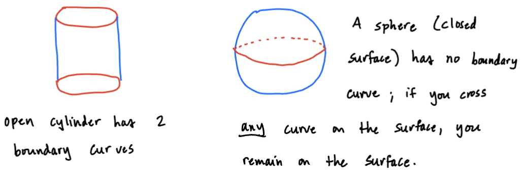
We will mainly be dealing with surfaces with one boundary curve with positive boundary orientation.

Recall the circulation form of Green’s Theorem:

\oint F \cdot d r = \int \int_{D} Q_{x} - P_{y} d A = \int \int_{D} c u r l (F) \cdot k d A

Where $\oint F \cdot d r$ is the circulation around boundary and $\int \int_{D} c u r l (F) \cdot k d A$ is the circulation throughout $D$

The circulation form of Green’s theorem tell us the circulation throughout a flat surface $D$ is equal to the line integral around the boundary of $D$ . Stokes’ Theorem generalizes this result to higher-dimensional surfaces

Stoke's Theorem (Fundamental theorem for the Curl)

Let $S$ be an oriented surface whose boundary curve $C$ has positive boundary orientation, and let $F$ be a vector field whose component functions have continuous partial derivatives. Then:
$\oint F \cdot d r = \int \int_{S} c u r l (F) \cdot d S$

Another way of stating Stokes’ Theorem:

\oint_{\partial S} F \cdot d r = \int \int_{S} (\nabla \times F) \cdot d S

where $\oint_{\partial S}$ is the boundary of $S$ and $(\nabla \times F)$ is the curl of $F$

Verbally

The circulation around the boundary of S is equal to the flux of the curl through S.

Moral

We can calculate a line integral as a flux integral

Proof of Stoke’s Theorem

We’ll do this for the special case where $S$ is the graph of a function, $z = f (x, y)$ , and

F = ⟨ P (x, y, z), Q (x, y, z), R (x, y, z)⟩

Set-up

Sketch

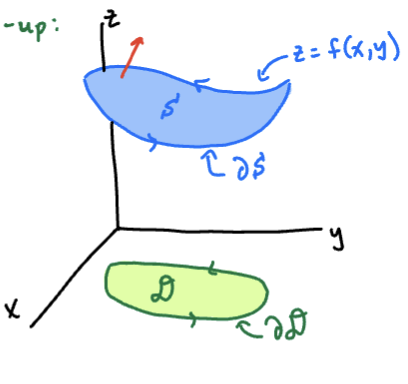
Parameterize $S$ by $r = ⟨ x, y, f (x, y)⟩$
Let $D$ be the projection of $S$ in the xy-plane. Parameterize $\partial D$ by:

\partial D : r_{1} (t) = ⟨ x (t), y (t)⟩, t \in [a, b]

Then a parameterization of $\partial S$ is found by “lifting” $\partial D$ up to $S$ :

\partial S : r_{2} = ⟨ x (t), y (t), f (x (t), y (t)) ⟩

We Must Show

\oint_{\partial S} F \cdot d r = \int \int_{S} c u r l (F) \cdot d S

1. Right-Hand Side of (*)

We have:

c u r l (F) = i \frac{\partial}{\partial x} P j \frac{\partial}{\partial y} Q k \frac{\partial}{\partial z} R = ⟨ R_{y} - Q_{z}, P_{z} - R_{x}, Q_{x} - P_{y} ⟩

$S$ has parameterization $⟨ x, y, f (x, y)⟩$ , so:

r_{x} \times r_{y} = i 10 j 01 k f_{x} f_{y} = ⟨ - f_{x}, - f_{y}, 1 ⟩ = ⟨ - z_{x}, - z_{y}, 1 ⟩

The surface integral is therefore:

\int \int_{S} c u r l (F) \cdot d S = \int \int_{D} ⟨ R_{y} - Q_{z}, P_{z} - R_{x}, Q_{x} - P_{y} ⟩ \cdot ⟨ - z_{x}, - z_{y}, 1 ⟩ d A = \int \int_{D} - (R_{y} - Q_{z}) Z_{x} - (P_{z} - R_{x}) Z_{y} + (Q_{x} - P_{y}) d A = \int \int_{D} (Q_{x} - P_{y}) + (Q_{z} - R_{y}) Z_{x} + (R_{x} - P_{z}) Z_{y} d A (* *)

2. Left-Hand Side of (*)

Using the parameterization of $\partial S$ on the previous page, we compute the line integral directly: $(r_{z} = ⟨ x (t), y (t), f (x (t), y (t))⟩)$

\oint_{\partial S} F \cdot d r = \int_{a}^{b} ⟨ P, Q, R ⟩ \cdot ⟨ d x, d y, d z ⟩ = \int_{a}^{b} [P x^{'} (t) + Q y^{'} (t) + R z^{'} (t)] d t

Observe
$z = f (x (t), y (t))$ , so by the chain rule:
graph TD
  z --> x
   z --> y
  x --> t["t"]
 y --> t2["t"]
$\frac{d}{d t} z (t) = Z_{x} X_{t} + Z_{y} Y_{t}$
Substituting and replacing $x^{'} (t) = X_{t}, y^{'} (t) = Y_{t}$ , yields:
$\oint_{\partial S} F \cdot d r = \int_{a}^{b} P x_{t} + Q y_{t} + R (Z_{x} X_{t} + Z_{y} Y_{t}) d t = \int_{a}^{b} (P + R z_{x}) X_{t} + (Q + R z_{y}) Y_{t} d t = \int_{a}^{b} ⟨ P + R z_{x}, Q + R z_{y} ⟩ \cdot ⟨ X_{t}, Y_{t} ⟩ d t$

Observe

This is a line integral around the curve $⟨ x (t), y (t)⟩$ , which is $\partial D$ , so by Green’s Theorem, we get:
$= \int \int_{D} \frac{\partial}{\partial x} (Q + R z_{y}) - \frac{\partial}{\partial y} (P + R z_{x}) d A (* * *)$

Recall: $P = P (x, y, z) = P (x, y, f (x, y))$ , so by the chain rule:

graph TD
   P --> x
   P --> y
   P --> z
   z --> x2["x"]
	z --> y2["y"]

\frac{\partial}{\partial y} P = P_{y} + P_{z} Z_{y}

By the Chain and Product Rules, the part of the integrand in (***) are:

(Q + R Z_{y})_{x} = Q_{x} + R_{x} Z_{y} + R Z_{y x} = (Q_{x} + Q_{z} Z_{x}) + (R_{x} + R_{z} Z_{x}) Z_{y} + R Z_{y x}

(P + R Z_{x})_{y} = P_{y} + R_{y} Z_{x} + R Z_{x y} = (P_{y} + P_{z} Z_{y}) + (R_{y} + R_{z} Z_{y}) Z_{x} + R Z_{x y}

Subtracting the 2nd from the 1st, using Clairut’s Theorem o the “end” terms, and going back into the integrand gives:

\int \int_{D} Q_{x} + Q_{z} Z_{x} + R_{x} Z_{y} + R_{Z} Z_{x} Z_{y} + R Z_{x y} - P_{y} - P_{z} Z_{y} - R_{y} Z_{x} - R_{z} Z_{x} Z_{y} - R Z_{x y} d A

= \int \int_{D} (Q_{x} - P_{y}) + (Q_{z} - R_{y}) Z_{x} + (R_{x} - P_{z}) Z_{y} d A

This equals the surface integral from step 1 exactly, verifying (*) and therefore proving the theorem. $□$

Remark

Observe that Green’s Theorem is a special case of Stokes’ Theorem. If $S$ is flat, $n = k$ , and
$\int_{\partial S} F \cdot d r = \int \int_{S} c u r l F \cdot n d S = \int \int_{S} c u r l F \cdot k d S$
Which is the circulation form of Green’s Theorem. $□$

Remark

We can finally prove:
$c u r l (F) = 0 \to F i s co n ser v a t i v e$
(So far, we’ve only proved $F$ conservative $\to c u r l F = 0$ .)

Proof

Let $C$ be any simple closed curve in $R^{3}$ . If $S$ is any surface with boundary curve $C$ , then by Stokes’:
$\oint F \cdot d r = \int c u r l F \cdot d S$
And, because $c u r l F = 0$ :
$= \int \int_{S} 0 d S = 0$
C was any simple closed curve, so $\oint F \cdot d r = 0$ for every simple closed curve $C$ . The result now falls like a stack of dominos: using results from sec. 16.3,
$\oint_{C} F \cdot d r = 0 f or a l l C \to \int_{C} F \cdot d r i s in d e p e n d e n t o f p a t h \to F i s co n ser v a t i v e ■$
( For non-simple closed curves, break up into a union of simple closed curves. )

Graph View

Stokes' Theorem

Verbally

Moral

Proof of Stoke’s Theorem

Set-up

We Must Show

1. Right-Hand Side of (*)

2. Left-Hand Side of (*)

Nearby

Similar, not linked

Explore