Reinforcement Learning

Machine Learning technique where comptuer programs ( often Neural Networks now through Policy Gradient Methods, see Proximal Policy Optimzation and other LLM based advancements ) learns to make choices through trial and error to reach some reward function.

We all know what RL is, this is just going to serve as a high level note on the theory behind it regarding Markov Decision Process

---

Main Markov Decision Process Loop

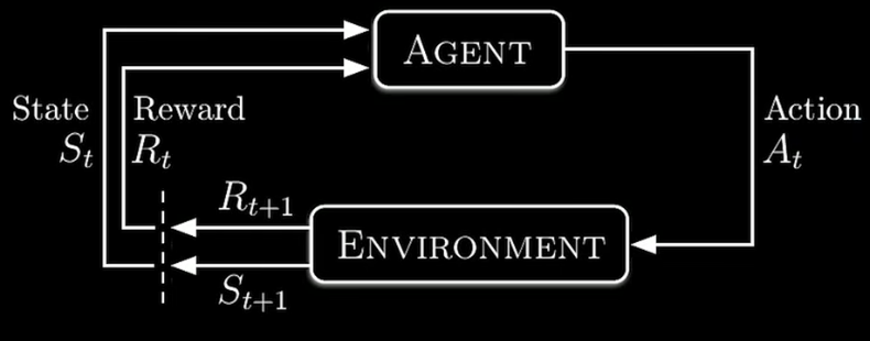
• Agent
  • represent that which learns and takes actions at each moment in time $T$
• Action
  • $A_t$ is received by environtment to produced reward and state for that moment in time
• Environtment
  • produces reward $R_{t+1}$ and a state $S_{t+1}$ at the next moment in time
• this is passed back to agent for next action to be decided

Time is discrete:

$$t\in \{0,1,2,\dots \}$$

then we have uppercase random variables $S,A,R$ for state action and reward, with lowercase values for the values they take $s,a,r$.

they are sets:

$$s\in \underset{\text{set can be anything here}}{\underbrace{S}}$$

the set $a$ belongs to dictates that the set of actions that $a$ can take depends on the current state that the agent is in.

$$a\in \underset{\text{depends on current state}}{\underbrace{\mathcal{A}(s)}}$$

and:

$$r\in \mathcal{R}\in \mathbb{R}$$

Dynamics of agent env interaction specified by distribution function:

$$\underset{\text{shorthand}}{\underbrace{p(s^{\prime },r\mid s,a)}}=Prob(S_{t+1}=s^{\prime },R_{t+1}=r\mid S_t=s,A_t=a)$$

this has the markov property, depends only on current state.

This defines the Finite Markov Decision Process, main objective of RL

Defining Behavior

We now have the policy, giving us the probability the agent will take a particurlar action when in a given state, likely a discrete probability distribution (could be continuous)

$$\pi (a\mid s)$$

if it is deterministic then its just:

$$a=\pi (s)$$

the goal of a policy is to accumulate a lot of a reward, which we call the return:

$$G_t=\stackrel{\text{this may sometimes be infinity}}{\overbrace{\sum _{k=t+1}^T}}{\gamma }^{k-t-1}{R}_k$$

just a sum of future reward, but because we want to favor sooner behavior rather than later, we add a discounting parameter $\gamma$, looks odd but just know that gamma when expanded means that rewards further away will have less weight:

$$R_{t+1}+\gamma R_{t+2}+{\gamma }^2{R}_{t+3}+\dots$$

we use $T$ because this assume that the loop will reach a terminal state, which for cases like this we refer to the set of states as ${\mathcal{S}}^{+}$

in this case, we can now define the goal as the policy that will maximize the expected return.

$${max}_{\pi }\mathbb{E}[G_t]$$

---

Example

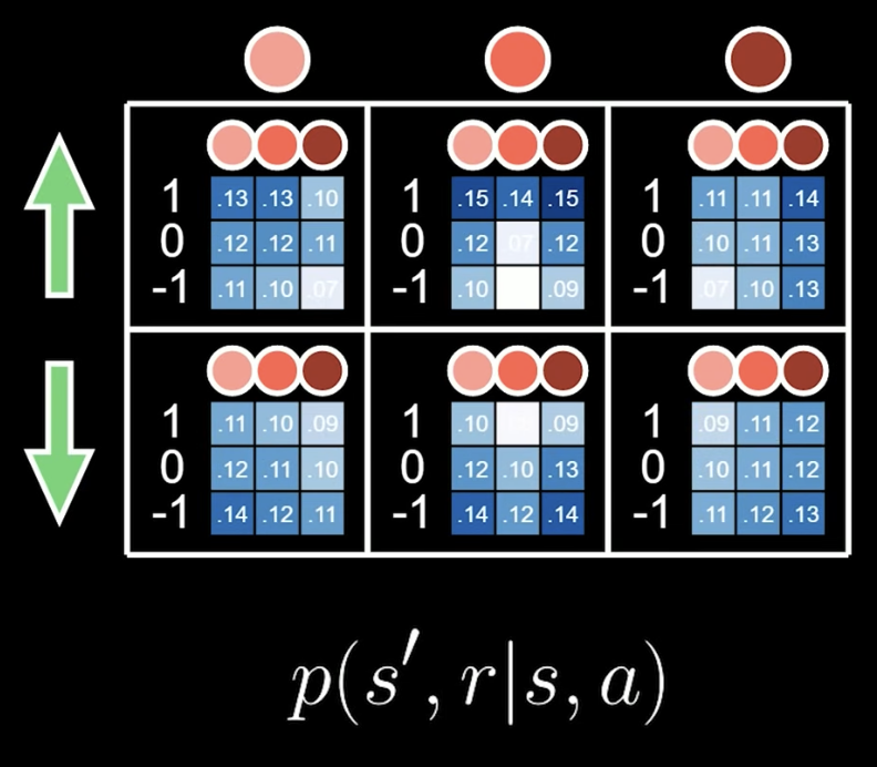
• Lets list out the different possible states $s$ as shades of red.
• in each state, an agent can take one of two actions $a$: up or down
  • this lays out the conditional part $p(s^{\prime },r\mid \underbrace{s,a})$

for each combination of state and action, we will have a distribution over the next state and reward

• lets say possible rewards $r$ are $\{-1,0,1\}$, and obviously the possible next states $s^{\prime }$ are the possible shades of red

we can picture these distributions as heatmaps:

State Value Function

v_{\pi}(s) = \underbrace{ \mathbb{E}_{\pi} [ G_{t} \mid S_{t} = s] }_{\begin{array} j \text{very similar to goal fuction} \\ max_{\pi} \mathbb{E}_{\pi} [ G_{t}] \end{array}}

Action Value Function

Defined similar, but also condition on the action

$$q_{\pi }(s,a)={\mathbb{E}}_{\pi }[G_t\mid S_t=s,A_t=a]$$

Warning

knowing these two functions in practice will typically be impossible! we will have to settle for estimates

what makes these useful? goal is to find the optimal policy ${\pi }_{\ast }$, which it turns out can be defined by their value functions:

$$v_{{\pi }_{\ast }}(s)\ge v_{\pi }(s)\text{for all s and for any }\pi$$

it is guarenteed there is always at least one optimal policy. same holds for value functions as well.

$$q_{{\pi }_{\ast }}(s,a)\ge q_{\pi }(s,a)\text{for all s,a and for any }\pi$$

Assumptions

• the agent observes $S_t$
• $S_t$ has the Markov Property

We sometimes assume

• Tabular: all states and actions can be listed
• Complete knowledge we have complete access to the envrionment’s dynamics
  • e.g. we have access to $p(s^{\prime },r\mid s,a)$

---

Policy Implementations

Big jump from prior guided learning writing, this part serves as an index of SOTA RL for mostly Large Language Model stuff.

Direct Policy Optimizatoin

• skips RL loop, instead deriving a closed form loss over preference pairs with the same optimum as KL constrained RLHF obj, thus you train directly on (chosen, rejected ) wtihout any sampling
  • quite cheap and stable, however off policy against a fixed dataset, thus thus can only reweight behavior that already appears within data.

Proximal Policy Optimzation

• clip importance ratio ${\pi }_{\theta }/{\pi }_{{\theta }_{old}}$ to $\left[1-ϵ,1+ϵ\right]$, so a single large advantage cant blow up the policy in a single update
• however needs a seperate value network, the Critic, to estimate $V(s)$, so roughly twice the parameters in memory during training
• default for Reinforcement Learning with Human Feedback for several years even InstructGPT, lot of surface to tune however: value head, GAE, cilp range, KL coefficient

Group Relative Policy Optimization

• we drop the critic entirely and instead take samples of group $G$ completions for same prompt and use groups own reward stats as the baseline, $A_i=\frac{r_i-mean(r)}{std(r)}$
  • much cheaper for this reason, and a great fit for RLVR since the only thing you need per completion is a scalar reward value.
  • has some failiure modes regarding length bias along with the std Normalization inflating advantage on groups where every sample scored about the same.
• created by deepseek and how deepseek r1 was trained.

Rewards

RLHF

• takes reward from a preference trained model, prefernce model is usually around the same size as the model being trained. Can be applied to anything however there is a tendancy for reward hacking as the reward model is only al earned approximation

RLVR

• takes reward from a checker, a lot more narrow in what it can be applied to ( popularity came from training LLMs for math and coding ), but the signal is rock solid and wont degrade unlike a reward model approximation.