Kalman Filter

A Kalman Filter is a tool for incorporating noisy measurements over time to estimate the true state of a dynamic system. It is widely used in control systems, robotics, and signal processing.

---

An Underlying Dynamical System Model

A great way to understand the Kalman Filter is to think of it as a hidden Markov model where the hidden states evolve over time according to a linear dynamical system, and the observations are noisy measurements of these states.

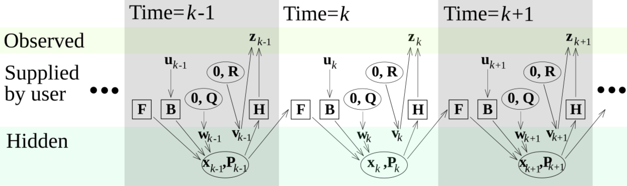
Model underlying the Kalman filter. Squares represent matrices. Ellipses represent multivariate normal distributions (with the mean and covariance matrix enclosed). Unenclosed values are vectors. For the simple case, the various matrices are constant with time, and thus the subscripts are not used, but Kalman filtering allows any of them to change each time step.

Where:

• ${\mathbf{F}}_k$ is the state transition model
• ${\mathbf{K}}_k$ is the observation model
• ${\mathbf{Q}}_k$ is the Covariance of the process noise
• ${\mathbf{R}}_k$ is the Covariance of the observation noise

---

The Kalman Filter Algorithm

The Kalman Filter operates in two stages: predict and update. At each time step $k$, we maintain an estimate of the state ${\hat{\mathbf{x}}}_k$ and its uncertainty (covariance) ${\mathbf{P}}_k$.

Prediction Step

First, we predict the next state based on the system dynamics:

$${\hat{\mathbf{x}}}_{k|k-1}={\mathbf{F}}_k{\hat{\mathbf{x}}}_{k-1|k-1}+{\mathbf{B}}_k{\mathbf{u}}_k$$ $${\mathbf{P}}_{k|k-1}={\mathbf{F}}_k{\mathbf{P}}_{k-1|k-1}{\mathbf{F}}_k^T+{\mathbf{Q}}_k$$

Where:

• ${\hat{\mathbf{x}}}_{k|k-1}$ is the a priori state estimate at step $k$ given observations up to $k-1$
• ${\mathbf{P}}_{k|k-1}$ is the a priori estimate covariance
• ${\mathbf{B}}_k$ is the control input model (often omitted if no control input ${\mathbf{u}}_k$)

Update Step

When we receive a measurement ${\mathbf{z}}_k$, we update our estimate:

First, compute the Kalman gain:

$${\mathbf{K}}_k={\mathbf{P}}_{k|k-1}{\mathbf{H}}_k^T({\mathbf{H}}_k{\mathbf{P}}_{k|k-1}{\mathbf{H}}_k^T+{\mathbf{R}}_k{)}^{-1}$$

Then update the state estimate:

$${\hat{\mathbf{x}}}_{k|k}={\hat{\mathbf{x}}}_{k|k-1}+{\mathbf{K}}_k({\mathbf{z}}_k-{\mathbf{H}}_k{\hat{\mathbf{x}}}_{k|k-1})$$

And the covariance:

$${\mathbf{P}}_{k|k}=(\mathbf{I}-{\mathbf{K}}_k{\mathbf{H}}_k){\mathbf{P}}_{k|k-1}$$

Where:

• ${\mathbf{K}}_k$ is the Kalman gain, determining how much to trust the measurement
• ${\mathbf{z}}_k-{\mathbf{H}}_k{\hat{\mathbf{x}}}_{k|k-1}$ is the innovation or measurement residual

---

Mathematical Intuition

Bayesian Perspective

The Kalman Filter is the optimal Bayesian estimator for linear-Gaussian systems. At each step, we’re computing:

$$p({\mathbf{x}}_k|{\mathbf{z}}_{1:k})\propto p({\mathbf{z}}_k|{\mathbf{x}}_k)\cdot p({\mathbf{x}}_k|{\mathbf{z}}_{1:k-1})$$

• Prior: $p({\mathbf{x}}_k|{\mathbf{z}}_{1:k-1})$ comes from the prediction step
• Likelihood: $p({\mathbf{z}}_k|{\mathbf{x}}_k)$ is the observation model
• Posterior: $p({\mathbf{x}}_k|{\mathbf{z}}_{1:k})$ is our updated belief after seeing ${\mathbf{z}}_k$

Because both distributions are Gaussian, their product is also Gaussian, and we can compute it in closed form.

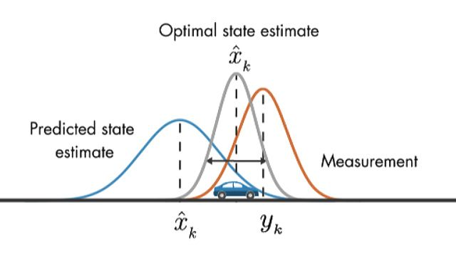
The Kalman Gain Intuition

The Kalman gain ${\mathbf{K}}_k$ balances trust between our prediction and the measurement:

• If measurement noise is small (${\mathbf{R}}_k$ small): ${\mathbf{K}}_k$ is large → trust the measurement more
• If prediction uncertainty is small (${\mathbf{P}}_{k|k-1}$ small): ${\mathbf{K}}_k$ is small → trust the prediction more

The update equation ${\hat{\mathbf{x}}}_{k|k}={\hat{\mathbf{x}}}_{k|k-1}+{\mathbf{K}}_k\cdot \text{(innovation)}$ can be read as:

“Start with our prediction, then correct it proportionally to how surprising the measurement was.”

Optimality

The Kalman Filter minimizes the mean squared error of the state estimate. It is provably optimal for linear systems with Gaussian noise. The covariance matrix ${\mathbf{P}}_k$ tracks our uncertainty, which typically decreases as we incorporate more measurements.

---

1D Example: Tracking Position

Consider a simple scenario: estimating the position of an object moving at constant velocity, given noisy position measurements.

Setup

State: ${\mathbf{x}}_k=\left[\begin{array}{c}\text{position}\\ \text{velocity}\end{array}\right]$

Dynamics (constant velocity):

$${\mathbf{x}}_k=\left[\begin{array}{cc}1& \Delta t\\ 0& 1\end{array}\right]{\mathbf{x}}_{k-1}+{\mathbf{w}}_k$$

where ${\mathbf{w}}_k\sim \mathcal{N}(0,\mathbf{Q})$ represents process noise.

Observation (we only measure position):

$$z_k=\left[\begin{array}{cc}1& 0\end{array}\right]{\mathbf{x}}_k+v_k$$

where $v_k\sim \mathcal{N}(0,R)$ is measurement noise.

Numerical Example

Let’s say:

• $\Delta t=1$ second
• Process noise: $\mathbf{Q}=\left[\begin{array}{cc}0.1& 0\\ 0& 0.1\end{array}\right]$
• Measurement noise: $R=4$ (quite noisy!)
• True trajectory: object starts at position 0, moving at 1 m/s

Initial state: ${\hat{\mathbf{x}}}_0=\left[\begin{array}{c}0\\ 0\end{array}\right]$, ${\mathbf{P}}_0=\left[\begin{array}{cc}5& 0\\ 0& 5\end{array}\right]$ (very uncertain)

Time step 1:

Predict:

• ${\hat{\mathbf{x}}}_{1|0}=\left[\begin{array}{cc}1& 1\\ 0& 1\end{array}\right]\left[\begin{array}{c}0\\ 0\end{array}\right]=\left[\begin{array}{c}0\\ 0\end{array}\right]$
• ${\mathbf{P}}_{1|0}=\left[\begin{array}{cc}1& 1\\ 0& 1\end{array}\right]\left[\begin{array}{cc}5& 0\\ 0& 5\end{array}\right]\left[\begin{array}{cc}1& 0\\ 1& 1\end{array}\right]+\left[\begin{array}{cc}0.1& 0\\ 0& 0.1\end{array}\right]=\left[\begin{array}{cc}10.1& 5\\ 5& 5.1\end{array}\right]$

Suppose we measure $z_1=1.5$ (true position is 1, but measurement is noisy).

Update:

• Innovation: $y_1=1.5-[10]\left[\begin{array}{c}0\\ 0\end{array}\right]=1.5$
• Innovation covariance: $S_1=[10]\left[\begin{array}{cc}10.1& 5\\ 5& 5.1\end{array}\right]\left[\begin{array}{c}1\\ 0\end{array}\right]+4=14.1$
• Kalman gain: ${\mathbf{K}}_1=\left[\begin{array}{cc}10.1& 5\\ 5& 5.1\end{array}\right]\left[\begin{array}{c}1\\ 0\end{array}\right]\frac{1}{14.1}\approx \left[\begin{array}{c}0.716\\ 0.355\end{array}\right]$
• Updated state: ${\hat{\mathbf{x}}}_{1|1}=\left[\begin{array}{c}0\\ 0\end{array}\right]+\left[\begin{array}{c}0.716\\ 0.355\end{array}\right]\cdot 1.5\approx \left[\begin{array}{c}1.07\\ 0.53\end{array}\right]$

Notice: the filter not only updated the position estimate but also inferred the velocity!

Visualization Interpretation

Over time, the Kalman Filter produces:

1. Smoother trajectory: The filtered estimate is less noisy than raw measurements
2. Decreasing uncertainty: The covariance ${\mathbf{P}}_k$ shrinks as more measurements arrive
3. Velocity inference: Even though we only measure position, the filter estimates velocity from the pattern of position changes

The filter balances:

• Physical model (constant velocity) vs. measurements
• High measurement noise ($R=4$) means trusting the model more
• As uncertainty decreases, the Kalman gain decreases, and updates become more conservative

This is why Kalman Filters are so powerful: they optimally fuse noisy data with a model of system dynamics to produce the best possible estimate.