The Bézier curve is a parametric curve often used for computer graphics. It is part of the family of spline curves, useful for defining paths using a set of control points.
The primary mechanism behind the Bézier curve is the Linear Interpolation function. Linear Interpolation takes in two points ( in the case of ) and can interpolate in between for a given parameter ( we are working with the parametric versions ):
Think of this as a function of time that will take in a value between and , and will return some point that resides on the line that those two points draw out:
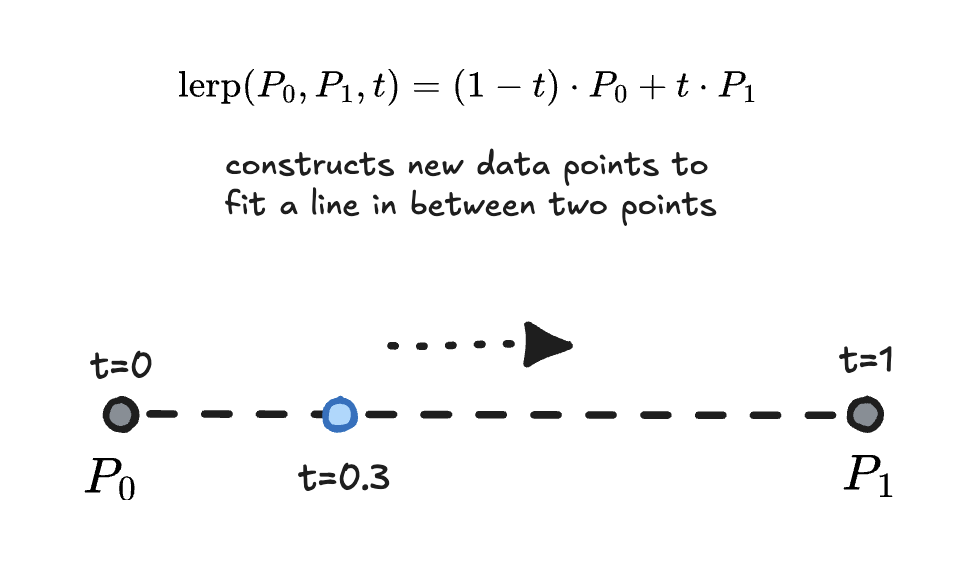
another possible definition for a LERP function
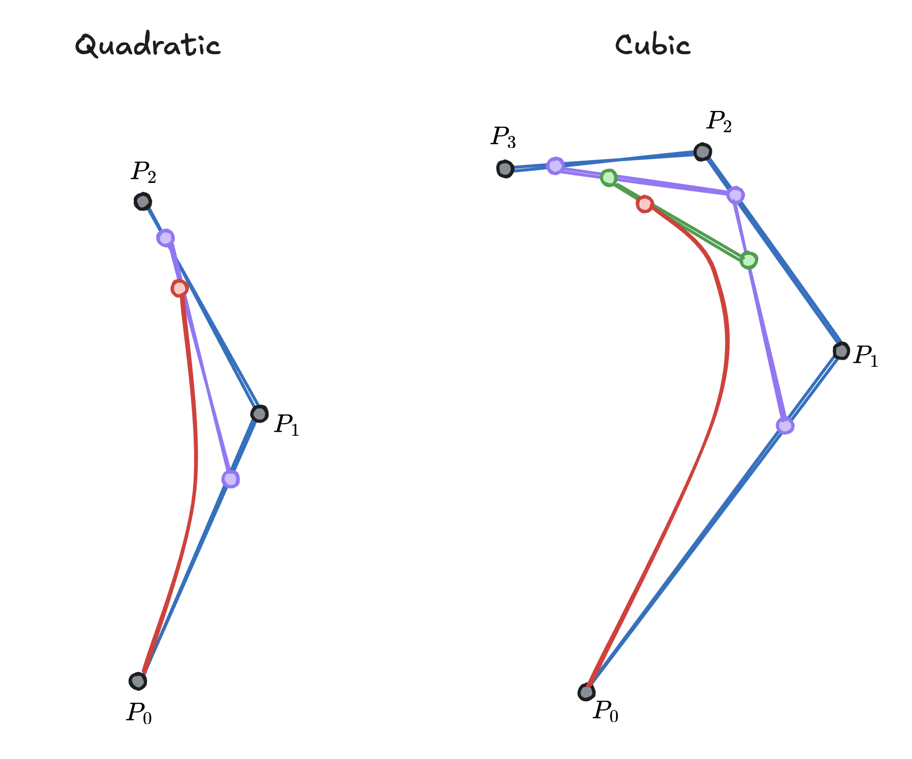
Interesting things occur when you have more than two points, and you then draw a new LERP line in between the outputted points of two previous LERPs.
This behavior, at least in the case of 3 points is what we call a quadratic bezier curve. This is because we have a degree of 2, and the outputted points are then used to create a new LERP line.
However the far more common case is the cubic bezier curve, which is defined by 4 points. The first and last points are the endpoints of the curve, while the two middle points are control points that define the curvature of the curve.
The cubic Bezier curve is the one most used in computer graphics, and is defined by the following equation:
Bernstein Polynomial Form
A more powerful way to express the cubic Bézier curve is using the Bernstein polynomial form:
A neat way to think of this is by visualizing each point as a vector from the origin to the point, and then scaling each vector by the polynomial coefficients. Adding these vectors together draws the same curve that running the LERP method would achieve.
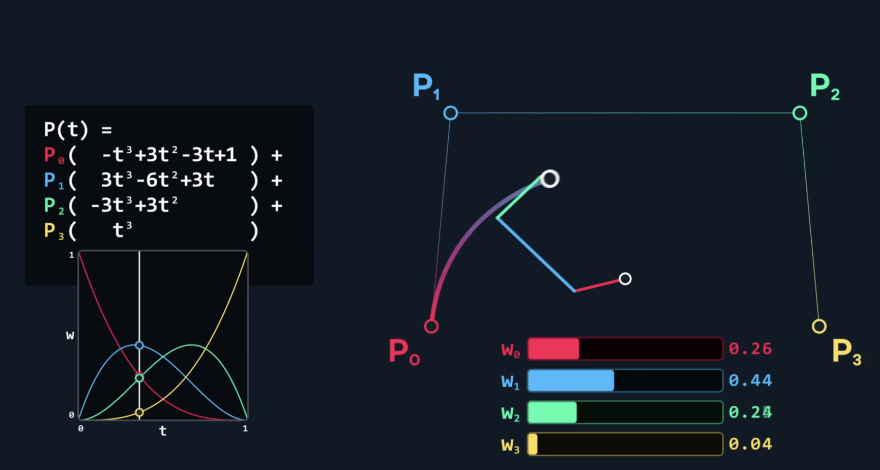
Lining the vectors up shows this sort of “wave” effect that the curve has, which is a result of the polynomial coefficients. This is a weighted sum, as all the values add up to one as they shift their weights.