Support Vector Machines

SVMs are good generalization classifiers both in theory and in practice. Particularly works well with few samples and high dimensional data.

The goal of the SVM algorithm is to find a hyperplane in an N-dimensional space (N — the number of features) that distinctly classifies the data points.

$$\text{Given a training dataset }\{(x_i,y_i){\}}_{i=1}^m,\text{ where }{x}_i\in {\mathbb{R}}^n\text{ and }{y}_i\in \{-1,1\},$$

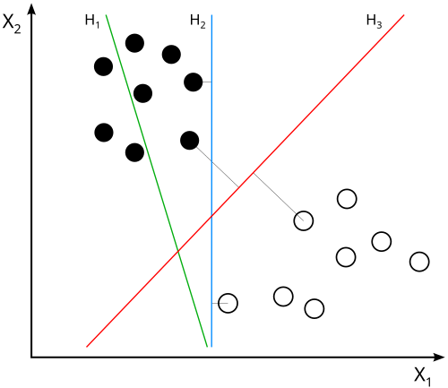
In plain english, they seek to find a “road” in the feature space that separates the two classes of data points with the largest possible margin. Not just a infitesimally thin line, but a wide road that gives some buffer room. Then, new data points can be classified based on which side of the road they fall on. Also allows for a “noise margin” where some points can be on the wrong side of the road if necessary.

$H_1$ does not separate the classes. $H_2$ does, but only with a small margin. $H_3$ separates them with the maximal margin.

---

Margin Classification

Margins serve to increase the classifier’s robustness to noise and improve generalization to unseen data.

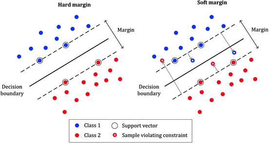
Hard margins will strictly impose all instances to be correctly classified, meaning no data points can fall within the margin or on the wrong side of the hyperplane.

While this approach can work well for linearly separable data, it is sensitive to outliers. A single misclassified point can drastically affect the position of the hyperplane, leading to poor generalization.

Soft margins are more flexible, allowing some data points to be within the margin or even misclassified. This is achieved by introducing slack variables that quantify the degree of misclassification for each data point.

---

Nonlinear SVMs

Linear SVMs work very well, however there will always be datasets that are not even close to being linearly separable. To handle such cases, SVMs can be extended to nonlinear decision boundaries using the kernel trick.

The trick we use is to “transform” the data and THEN apply a linear SVM in this transformed space. The transformation is done using a kernel function, which computes the inner product of the data points in the transformed space without explicitly performing the transformation.

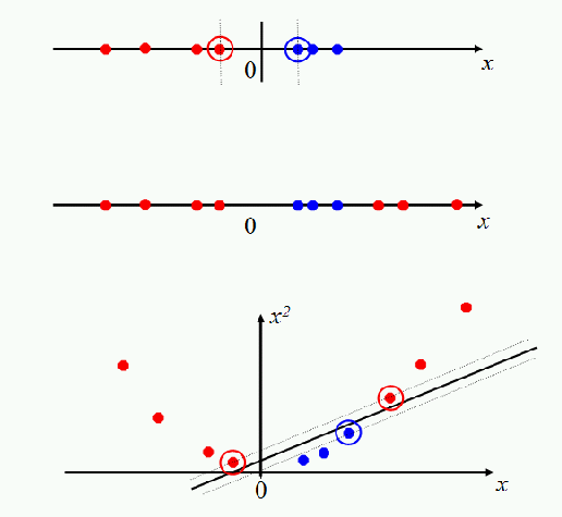
The classic case as seen above is the squaring, where the transformation is $\varphi (x_1,x_2)=(x_1^2,\sqrt{2}{x}_1{x}_2,x_2^2)$.

This has allowed for that clump in the middle to have an extra dimension which the linear SVM can then separate.

Kernel Methods

The kernel function $K(x_i,x_j)$ computes the inner product of the transformed data points $\varphi (x_i)$ and $\varphi (x_j)$ in the higher-dimensional space:

$$K(x_i,x_j)=⟨\varphi (x_i),\varphi (x_j)⟩$$

Gaussian (RBF) Kernel

Another common transformation is the Gaussian or Radial Basis Function (RBF) kernel, which maps data into an infinite-dimensional space. The RBF kernel is defined as:

$$K(x_i,x_j)=\exp \left(-\frac{\Vert x_i-x_j{\Vert }^2}{2{\sigma }^2}\right)$$

We use something called “landmarks” to represent the data in this infinite-dimensional space. Each landmark corresponds to a training example, and the features are computed based on the similarity to these landmarks using the RBF kernel.

Other Kernels

Cosine Similarity Kernel: for text data, measures the cosine of the angle between two vectors.

Sigmoid Kernel: resembles the behavior of neural networks, defined as $K(x_i,x_j)=\tanh (\alpha ⟨x_i,x_j⟩+c)$.

Chi-Squared Kernel: often used in image classification tasks, particularly with histogram data.