We return to A short history of AI, were we had a brief look at Braitenberg Vehicles. While we learned about how the inputs and outputs connected to form emergent behavior, we now need to generalize the concept of “neurons” and “connections” to build more complex systems.
Neural Networks
Few terms to introduce:
- Pre-synaptic neuron: the neuron sending the signal
- Post-synaptic neuron: the neuron receiving the signal
- Neuron activation: the level of activity of a neuron, often represented as a number between 0 and 1
- Synapse: the connection between two neurons.
In more standard machine learning, we just refer to these as “neurons” and “connections”.
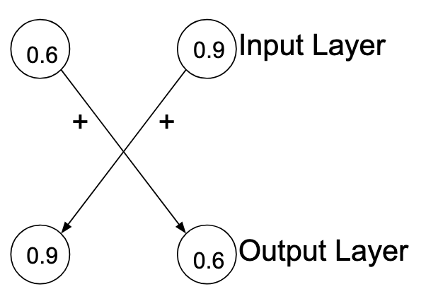
In the case of the Braitenberg vehicles, we had 4 neurons, two inputs and two outputs. There were no “deep” layers or connections, and all the connections did was “criss cross” the inputs and outputs with a particilar weight.
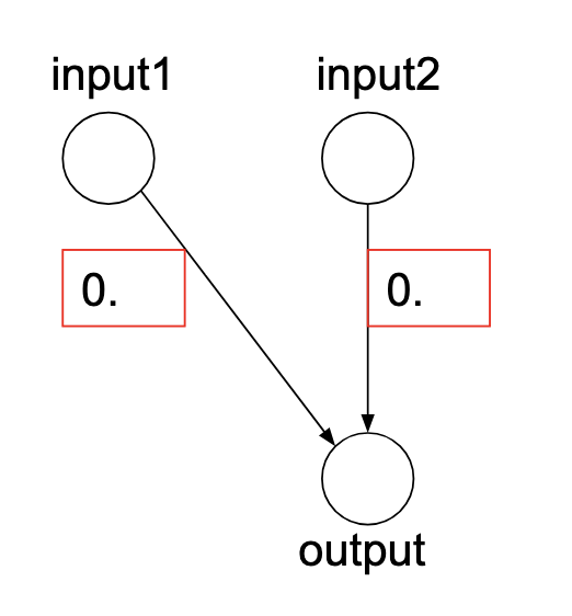
In more traditional neural networks, we usually see the previous layer neurons have a connection to every single neuron in the next layer. We then let training tune the weights of these connections to produce the desired output.
There are two “tunable” parameters for each connection:
- Weight: Parameter for the connection between the pre-synaptic and post-synaptic neuron. This determines how much influence the pre-synaptic neuron has on the post-synaptic neuron. It is a multiplicative factor.
- Bias: This is an additive parameter that gets added to the sum of all the weighted inputs to the post-synaptic neuron. It allows us to shift the activation function left or right, which can be crucial for learning.
We then apply the activation function to the weighted sum of inputs plus bias to determine the final output of the post-synaptic neuron.
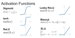
Activation Functions
This is were things get a bit more novel. In the case of the Braitenberg vehicles, the activation function was simply linear - the more input you had, the more output you got. However, in more complex neural networks, we often use non-linear activation functions to introduce complexity and allow the network to learn more intricate patterns.
What Neural Networks DO
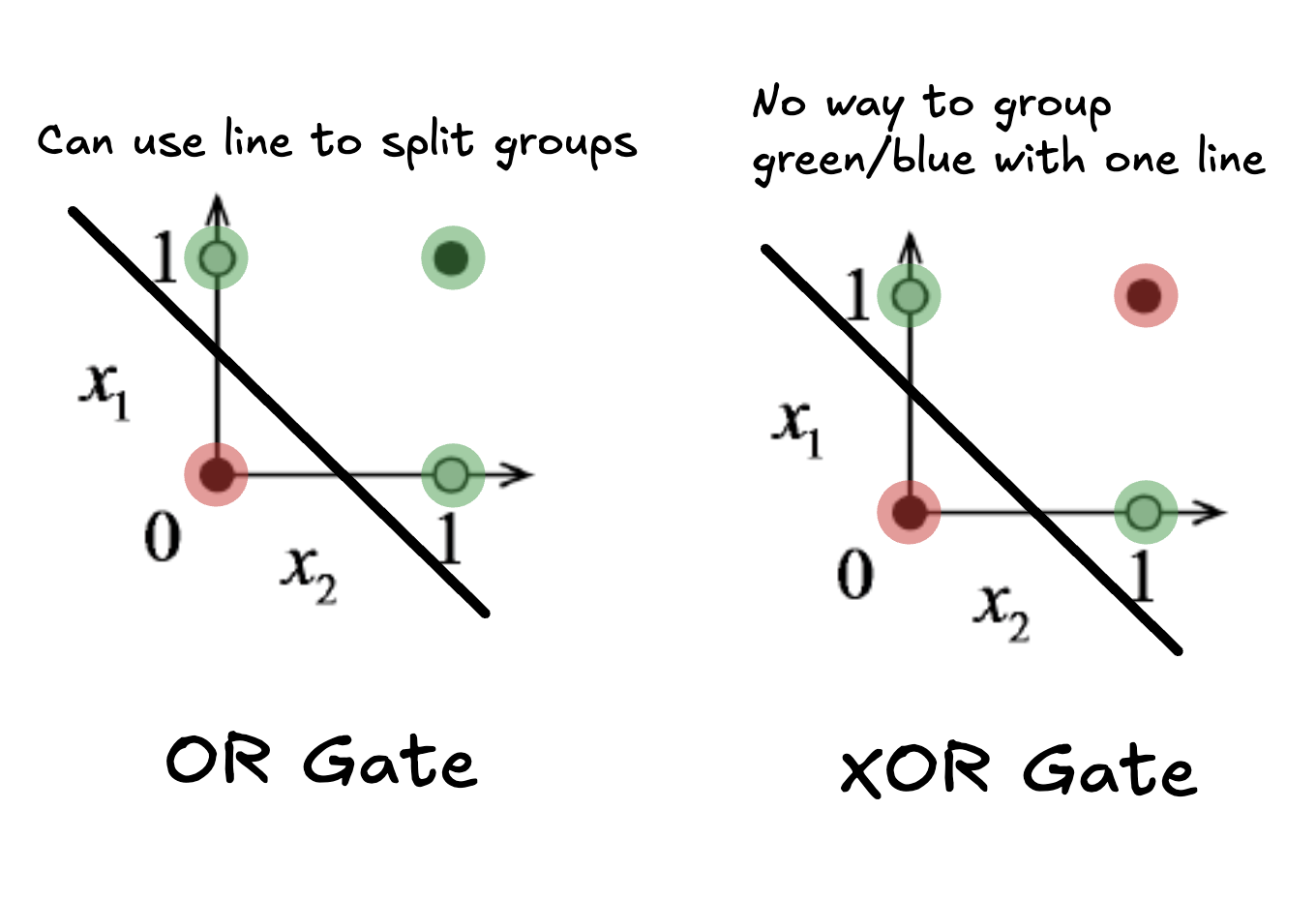
The most basic example is those of the logic gates, with two inputs and one output. By adjusting the weights and biases, we can create networks that behave like AND, OR, and NOT gates.
The best way to think about these shallow networks is as a linear “fold”, where one side is classified as a 0 and the other as a 1. It is quite literally just a line drawn on a 2D plane at this scale.
Why XOR is Hard
If you think about the plot of the two inputs on the 2d plane, you can imageine the line that would be drawn to classify all the other gates. But, in this case, there is no single line you can draw to seperate the 1s from the 0s. This is why we need deeper networks with more layers to solve more complex problems.
Backpropagation
Quite a heavy concept that we wont discuss implementation on (unless you are in the Grad group), but in essence, backpropagation allows us to learn synaptic weights and biases through training. A rough description would be it calculating the “incorrectness” of the output(called a Loss Function), finding the “rate of change” of the loss with respect to each weight and bias(partial derivatives), and then taking a step in the direction it belives will reduce the loss(the negative gradient). Think of a ball rolling down a hill, where the steepest direction is the direction of the negative gradient.
Map sucess to a “hily field” of weights and biases, and then roll down the hill to find the best set of weights and biases.
Weakness Of Backpropagation
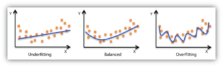
Unfortunately backpropagation is prone to a new issue: overfitting. This is where the network learns the training data too well, and fails to generalize to new data. This is a common problem in machine learning, and there are various techniques to mitigate it, such as regularization, dropout, and early stopping.
This usually happens when the network starts trying to learn the noise of the data, rather than the latent distribution. There are some techniques using bayesian probability theory called Variational Inference that treat noise as a probability distribution to be modeled, rather than a set of points to be learned.