Forced Damped Pendulum

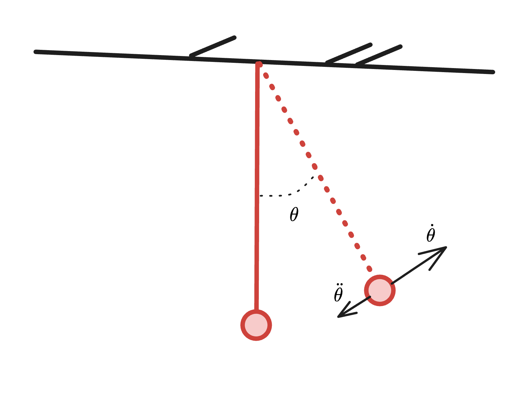
We start the lecture with the introduction with a forced damped pendulum.

Much like pendulum phase space visualizations seen in 3Blue1Brown, we plot the angle $\theta$ as the $x$ axis and the angular velocity $\dot{\theta }$ as the y axis.

• the difference in this case is that there is an external force being applied sinusoidally, meaning the force applied varies from left to right as a sin signal.

Chaotic Forced Damped Pendulum

The very interesting thing about this chaotic system is that instead of the Fixed Points being single values that the Logistic Map converges on, we instead see a whole continuum of points that the system converges on.

We dont converge on a point, we converge on a flow. It feels something of the sort of abstraction of rate of change from calculus, where we are not concerned with the value of a function at a point, but rather the behavior of the function in the neighborhood of that point.

But much like the Logistic Map, there are parameters we can tune to make this system no longer converge on this flow, and will remain chaotic forever.

How are we defining "flow" here?

In the subject of this class, we look for the period of time it takes for a system to return to its original state. Then for any given system, we look at a certain time point and the next period of that repetitive time point. In the case of the forced damped pendulum, we look at the state of the system every time the forcing function completes a full cycle.

In essence, we are just taking a snapshot every $2\pi$ that converts the flow space into a single point.

---

Defining the Force Damped Pendulum

The differential equation for the pendulum remains quite standard:

$$\frac{d^2\theta }{d{t}^2}+b\frac{d\theta }{dt}+c\sin (\theta )=F\sin (\omega t)$$

But our difference is defining the added force as passing through an oscillatory function, in this case a sine wave.

$$\text{Force}=F\sin (\omega t)$$

Simulating this equation numerically, we treat the second order ode as a system of first orders.

We also have the following two parameters to “play around with”

• $\theta$ : angular position (radians)
• ${\omega }_{\theta }=\frac{d\theta }{dt}$ : angular velocity (radians/second)

Our two first order ODEs:

$$\begin{array}{rl}\frac{d\theta }{dt}& ={\omega }_{\theta }\\ \frac{d{\omega }_{\theta }}{dt}& =-b{\omega }_{\theta }-c\sin (\theta )+F\sin (\omega t)\end{array}$$

Where:

• $b$ : damping coefficient (friction, air resistance)
• $c$ : gravitational constant term, typically $c=\frac{g}{L}$ where $g$ is gravitational acceleration and $L$ is pendulum length
• $F$ : amplitude of the external forcing
• $\omega$ : angular frequency of the external forcing (radians/second)
• $t$ : time

The Forcing Function:

$$F_{\text{external}}(t)=F\sin (\omega t)$$

This periodic forcing is what drives the system and, depending on parameter values, can produce chaotic behavior. The forcing frequency $\omega$ and amplitude $F$ are the key tunable parameters that determine whether the system exhibits regular periodic motion or chaotic dynamics.

---

A famous plot is that of the parameter space. There is a quite popular 2swap video made with his library Swaptube, where you parameterized the initial conditions and color by how long it takes to converge/diverge:

see “Double Pendulums are Chaos’nt” for a great visual

---

Two Dimensional Maps

The Hėnon Map:

$$f(x,y)=(a-x^2+by,x)$$

Showed that quadratic maps of the plane can exhibit the same behavior as Poìncaré Maps for ODEs. (e.g., forced damped pendulum, or N-body simulations of gravity)

Hėnon discovered that for certain values of $a$ and $b$, the map exhibits chaotic behavior, leading to the famous Hėnon attractor.

How to Use the Hėnon Map

The Hėnon map is an iterative function that takes a point in the plane $(x,y)$ and maps it to a new point $(x^{\prime },y^{\prime })$ using the transformation:

$$\begin{array}{rl}{x}_{n+1}& =a-x_n^2+b{y}_n\\ y_{n+1}& =x_n\end{array}$$

Classic Parameter Values:

• $a=1.4$
• $b=0.3$

These values produce the famous Hėnon attractor, a strange attractor with fractal structure.

Iterations are perfomed with the following process:

1. Start with an initial point $(x_0,y_0)$
2. Apply the transformation repeatedly
3. After transient behavior settles (typically discard first 100-1000 iterations), the remaining points trace out the attractor
4. The system exhibits sensitive dependence on initial conditions, a hallmark of chaos

Poìncaré Maps are a technique used to analyze continuous dynamical systems by taking snapshots of the system at regular intervals, much like our initial interpretations of how to map the “flow” to points.

Take a Poincaré section of the pendulum (sampling at regular intervals of the forcing period), we reduce the continuous flow to a discrete map, this is similar to how the Hėnon map operates.

Visualizing the Hėnon Attractor

Python

import numpy as np import matplotlib.pyplot as plt def henon_map(x, y, a=1.4, b=0.3): x_next = a - x**2 + b*y y_next = x return x_next, y_next def plot_henon_attractor(a=1.4, b=0.3, n_iterations=10000, n_discard=100): x, y = 0.1, 0.1 x_points = [] y_points = [] for _ in range(n_discard): x, y = henon_map(x, y, a, b) for _ in range(n_iterations): x, y = henon_map(x, y, a, b) x_points.append(x) y_points.append(y) fig, ax = plt.subplots(figsize=(10, 8), facecolor='black') ax.set_facecolor('black') ax.scatter(x_points, y_points, s=0.1, c='cyan', alpha=0.5) ax.set_xlabel('x', color='white', fontsize=12) ax.set_ylabel('y', color='white', fontsize=12) ax.set_title(f'Hénon Attractor (a={a}, b={b})', color='white', fontsize=14, pad=20) ax.tick_params(colors='white') ax.spines['bottom'].set_color('white') ax.spines['top'].set_color('white') ax.spines['left'].set_color('white') ax.spines['right'].set_color('white') plt.tight_layout() plt.show() plot_henon_attractor(a=1.4, b=0.3, n_iterations=50000, n_discard=500)

Output

Try different param values and see how they change the plot:

• For $a=1.4,b=0.3$: Classic strange attractor
• For $a=1.3,b=0.3$: Different attractor shape
• For $a=1.2,b=0.3$: Period-7 orbit (periodic, not chaotic)
• As you vary $a$, you can observe bifurcations similar to the Logistic Map

---

Example

Forced, Damped Pendulum: $a=\frac{F}{m}$,

$$\ddot{\theta }=\underset{\text{friction}}{\underbrace{-c\dot{\theta }}}-\underset{\text{gravity}}{\underbrace{\sin \theta }}+\underset{\text{forcing}}{\underbrace{\rho \sin t}}$$

Parameters are $c,\rho$