If we want to show that has chaotic orbits, we will do it by comparing with ( our Tent Map ).
For each point in the Tent Map domain , there is a companion point in the domain of that imitates its dynamics.
We say the maps and are conjugate if they are related by a continuous one to one change of coordinates.
Example
or
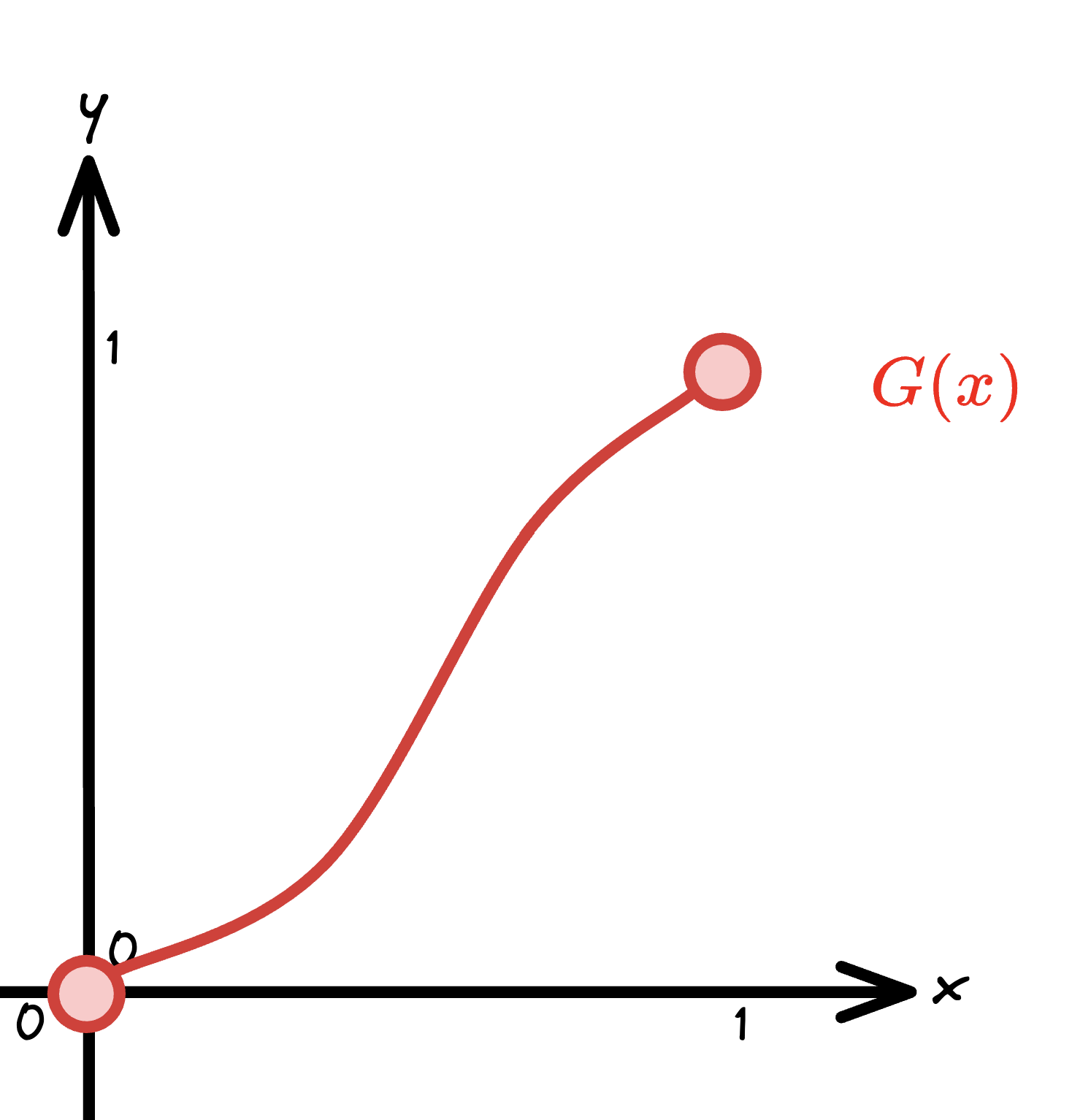
The maps and are conjugate by:
and:
For :
Idea
Two ways of getting from domain of to range of after iterations:
Evaluate directly — expensive, analytically intractable for large
Use conjugacy: since , induction gives , so:
Map into T’s domain via , iterate the simpler tent map times, then map back. Orbit structure of is exactly that of , just seen through the lens .
Suppose for a Fixed Point and then:
So stability of Fixed Point of and stability of Fixed Point , for are the same
Transition Graphs
Theorem (Covering implies fixed point)
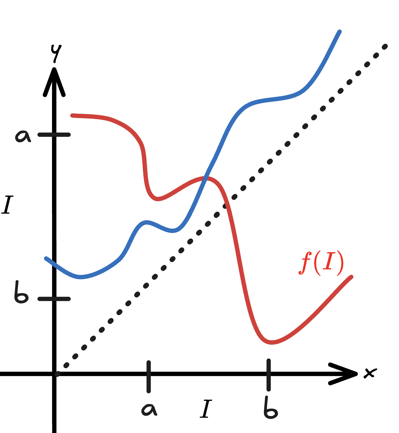
The blue line in the figure is the counterexample — a function where , so IVT doesn’t force a fixed point.
In topology, the general version is Brouwers Fixed Point Theorem.
Setup
A partition of the interval is a collection of subintervals that are pairwise disjoint (except at endpoints) whose union is the whole interval.
For both and , the natural partition is :
Definition: Draw an arrow in the transition graph if and only if — ” of covers “.
The covering condition matters because: if , then by the Intermediate Value Theorem there exists a point in that maps into . Covering arrows are existence guarantees for orbits.
Computing the Graph for
The Tent Map with :
- and
- and
All four arrows exist. The Tent Map transition graph is completely connected.
By conjugacy, has the same graph — also maps both and surjectively onto .
A path of length in the graph is a sequence where each arrow is a valid transition. This corresponds to an admissible itinerary; there genuinely exists a point whose orbit visits in order.
Consequence of complete connectivity: Every infinite sequence over is admissible. That’s an uncountable family of distinct symbolic trajectories, each encoding a genuinely different orbit.
Periodic orbits from cycles: A cycle of length in the graph (e.g. returning to ) guarantees a period- orbit exists in that sequence of intervals. Since all arrows exist, cycles of every length exist → infinitely many periodic orbits.